Content from Перед тим як почати

---

Last updated on 2026-01-19 | Edit this page

Estimated time: 40 minutes

Instructor Note

• Основна мета цього епізоду - допомогти слухачам комфортно почуватися під час користування інтерфейсом RStudio.
• У епізоді “Початкове налаштування” виконуйте усі етапи дуже повільно. Переконайтеся, що всі учасники встигають за ходом заняття (нагадайте їм користуватися наліпками для зворотного зв’язку). На цьому етапі домовтеся з помічниками, щоб вони ходили по аудиторії та допомагали учасникам. Дуже важливо впевнитися, що всі працюють у правильному робочому каталозі та створили підкаталог data (усі літери малі).

Overview

Questions

• Як орієнтуватися в RStudio?
• Як взаємодіяти з R?
• Як керувати робочим середовищем?
• Як встановити пакети?

Objectives

• Встановити останню версію R.
• Встановити останню версію RStudio.
• Ознайомитися з інтерфейсом RStudio.
• Встановити додаткові пакети за допомогою вкладки “packages”.
• Встановити додаткові пакети за допомогою команд R.

Що таке R? Що таке RStudio?

---

Термін “R” використовується як для позначення мови програмування, так і для програмного забезпечення, яке виконує скрипти, написані цією мовою.

RStudio нині є дуже популярним середовищем не тільки для написання скриптів на R, але й взаємодії з програмним забезпеченням R. Для правильної роботи RStudio потребує R і тому обидва необхідно встановити на ваш комп’ютер.

Щоб полегшити роботу з R, ми будемо використовувати RStudio. RStudio є найпопулярнішим IDE (інтегроване середовище розробки) для R. IDE - це частина програмного забезпечення, яка надає інструменти для полегшення програмування.

Також ви можете використовувати функцію R Presentations, щоб представляти свою роботу у вигляді презентації HTML5, поєднуючи Markdown і код на R. Ви можете переглядати їх безпосередньо в R Studio або у браузері. Є багато варіантів налаштування слайдів презентації, зокрема можливість зображати рівняння у форматі LaTeX. Це може допомогти вам співпрацювати з іншими, а також застосовувати для викладання та використання в класі.

Навіщо вивчати R?

---

У R не потрібно багато клацати мишкою — і це добре

Крива навчання може бути крутішою, ніж в інших програм, але в R результати аналізу залежать не від того, чи ви запам’ятали послідовність клацань мишкою, а від написаних команд — і це добре! Тому, якщо ви хочете повторити аналіз після того, як зібрали більше даних, вам не потрібно згадувати, у якому порядку ви натискали кнопки, щоб отримати результат — достатньо просто знову запустити свій скрипт.

Робота зі скриптами робить кроки вашого аналізу зрозумілими, а написаний вами код може переглянути інша людина, щоб дати відгук і помітити помилки.

Робота зі скриптами змушує вас глибше розуміти те, що ви робите, і допомагає краще вивчати та усвідомлювати методи, які ви використовуєте.

Код R сприяє відтворюваності

Відтворюваність — це коли інша людина (або навіть ви в майбутньому) може отримати ті самі результати з того самого набору даних, використовуючи той самий аналіз.

R інтегрується з іншими інструментами, щоб створювати публікації прямо з вашого коду. Якщо ви зберете більше даних або виправите помилку в наборі даних, графіки та статистичні тести у вашому документі оновляться автоматично.

Все більше журналів і грантодавців очікують, що аналізи будуть відтворюваними, тож знання R дає вам перевагу для виконання цих вимог.

Щоб ще більше підтримати відтворюваність і прозорість, існують пакети, які допомагають керувати залежностями: відстежувати, які пакети ми завантажуємо і як вони залежать від версії пакета, яку ви використовуєте. Це допомагає переконатися, що наявні робочі процеси працюють стабільно й продовжують виконувати те саме, що й раніше.

Такі пакети, як renv, дозволяють “зберігати” й “завантажувати” стан бібліотеки вашого проєкту, а також відстежують версії пакетів, які ви використовуєте, і джерело, з якого їх можна отримати.

R є міждисциплінарним і розширюваним

Маючи понад 10,000+ пакетів, які можна встановити для розширення її можливостей, R забезпечує середовище, що дозволяє поєднувати статистичні підходи з різних наукових дисциплін і підібрати саме ту аналітичну структуру, яка найкраще підходить для аналізу ваших даних. Наприклад, у R є пакети для аналізу зображень, GIS, часових рядів, популяційної генетики та багато іншого.

R працює з даними будь-яких форм і розмірів

Навички, які ви здобуваєте в R, легко масштабуються разом із розміром вашого набору даних. Незалежно від того, чи має ваш набір даних сотні чи мільйони рядків, це не матиме особливого значення для вас.

R призначений для аналізу даних. У R є спеціальні структури даних і типи даних, які роблять роботу з пропущеними значеннями та статистичними факторами зручною.

R може підключатися до електронних таблиць, баз даних та багатьох інших форматів даних — як на вашому комп’ютері, так і в інтернеті.

R створює високоякісну графіку

Можливості побудови графіків у R практично безмежні й дозволяють налаштувати будь-який аспект графіка, щоб якнайкраще передати зміст ваших даних.

R має велику та привітну спільноту

Тисячі людей використовують R щодня. Багато з них готові допомогти вам через списки розсилки та вебсайти, такі як Stack Overflow, або на спільноті RStudio. Питання, які супроводжуються короткими, відтворюваними фрагментами коду, швидше за все, отримують компетентні відповіді.

R не лише безплатна, вона також є з відкритим кодом і працює на різних операційних системах

Кожен може переглянути вихідний код, щоб побачити, як працює R. Завдяки такій прозорості менше шансів на помилки, а якщо ви (або хтось інший) їх знайдете — можна повідомити про них і виправити.

Оскільки R є відкритим кодом і підтримується великою спільнотою розробників та користувачів, існує дуже великий вибір сторонніх додаткових пакетів, які безплатно розширюють базові можливості R.

RStudio розширює можливості R та спрощує написання коду і взаємодію з R. Автор фото зліва; Автор фото справа.

Огляд RStudio

---

Знайомство з RStudio

---

Почнемо з вивчення RStudio, який є інтегрованим середовищем розробки (IDE) для роботи з R.

Відкрита версія RStudio IDE є безплатною за Загальна публічна ліцензія Affero (AGPL) v3. RStudio IDE також доступна з комерційною ліцензією та пріоритетною email-підтримкою від RStudio, Inc.

Ми будемо використовувати RStudio IDE для написання коду, роботи з файлами на комп’ютері, перегляду створених змінних і візуалізації побудованих графіків. RStudio також можна використовувати для інших речей (наприклад, контролю версій, розробки пакетів, створення Shiny-застосунків), які ми не розглядатимемо під час цього курсу.

Однією з переваг використання RStudio є те, що вся інформація, необхідна для написання коду, доступна в одному вікні. Крім того, RStudio надає багато комбінацій клавіш, автодоповнення та підсвічування синтаксису для основних типів файлів, які ви використовуєте під час роботи в R. RStudio робить набір коду простішим і менш схильним до помилок.

Налаштування

---

Це хороша практика зберегти набір пов’язаних даних, аналіз і текст самою текою під назвою робочий каталог. Усі скрипти у цій теці можуть потім використовувати відносні шляхи до файлів. Відносні шляхи вказують, де саме всередині проєкту знаходиться файл (на відміну від абсолютних шляхів, які показують розташування файлу на конкретному комп’ютері). Такий спосіб роботи значно полегшує перенесення вашого проєкту на інший комп’ютер або обмін ним з іншими, без потреби змінювати шляхи до файлів у кожному окремому скрипті.

RStudio надає зручні інструменти для цього через інтерфейс “Проєкти”, який не лише створює для вас робочий каталог, але й запам’ятовує її розташування (що дозволяє швидко повертатися до неї). Цей інтерфейс також (за бажанням) зберігає ваші налаштування та відкриті файли, щоб вам було легше продовжити роботу після перерви.

Створення нового проєкту

• У меню File (файл) натисніть New project (новий проєкт), виберіть New directory (новий каталог), потім New project (новий проєкт)
• Введіть назву цієї нової теки (або “каталогу”) і виберіть зручне розташування для неї. Це буде ваш робочий каталог до кінця дня (наприклад, ~/data-carpentry)
• Натисніть Create project (створити проєкт)
• Створіть новий файл, у якому ми будемо писати наші скрипти. Перейдіть до File (файл) > New File (новий файл) > R script (скрипт R). Натисніть значок збереження на панелі інструментів і збережіть ваш скрипт як “script.R”.

Найпростіший спосіб відкрити проєкт RStudio після його створення - це перейти до теки, де збережено проєкт і двічі клацнути на файлі .Rproj (синій куб). Це відкриє RStudio і запустить вашу сесію R у тому самому каталозі, де знаходиться файл .Rproj. Усі ваші дані, графіки та скрипти тепер будуть відносними до каталогу проєкт. Проєкти RStudio мають додаткову перевагу: вони дозволяють відкривати кілька проєктів одночасно, кожен у власному каталозі проєкту. Це дозволяє тримати відкритими кілька проєктів одночасно, не заважаючи один одному.

Інтерфейс RStudio

Давайте швидко ознайомимося з RStudio.

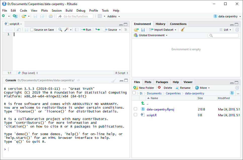
RStudio поділено на чотири “панелі”. Розміщення цих панелей та їх вміст можна налаштувати (див. меню, Tools (Інструменти) -> Global Options (Глобальні параметри) -> Pane Layout (Макет панелі)).

Макет за замовчуванням:

• Ліворуч вгорі - Source: ваші скрипти та документи
• Ліворуч унизу - Console: як виглядав би R без RStudio
• Праворуч угорі - Environment/History: тут можна побачити, що ви зробили
• Праворуч унизу - Files і інші вкладки: тут можна переглядати вміст проєкту/робочого каталогу, наприклад ваш файл Script.R

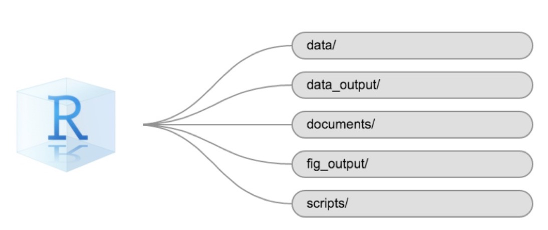
Організація робочого каталогу

Використання послідовної структури тек у всіх ваших проєктах допоможе підтримувати порядок і полегшить знаходження та збереження файлів у майбутньому. Це може бути особливо корисним, коли у вас є кілька проєктів. Загалом, ви можете створити каталоги (теки) для скриптів, даних та документів. Ось - кілька прикладів запропонованих каталогів:

• data/ Використовуйте цю теку для зберігання необроблених даних та проміжних наборів даних. З метою прозорості та походження, ви повинні завжди зберігати копію ваших необроблених даних доступною та максимально виконувати очищення й попередню обробку даних програмно (тобто за допомогою скриптів, а не вручну), наскільки це можливо.
• data_output/ Коли вам потрібно змінити необроблені дані, може бути корисно зберігати змінені версії наборів даних в іншій теці.
• documents/ Використовується для контурів, чернеток та іншого тексту.
• fig_output/ Ця тека може зберігати графіку, створену вашими скриптами.
• scripts/ Місце для зберігання ваших R-скриптів для різних аналізів або побудови графіків.

Вам можуть знадобитися додаткові каталоги або підкаталоги залежно від потреб вашого проєкту, але вони повинні складати основу вашого робочого каталогу.

Робочий каталог

Робочий каталог - важливе поняття для розуміння. Це місце, де R буде шукати та зберігати файли. Коли ви пишете код для свого проєкту, ваші скрипти повинні посилатися на файли відносно кореня робочої директорії й лише на файли в межах цієї структури.

Використання проєктів RStudio полегшує роботу і гарантує належне налаштування робочого каталогу. Якщо вам потрібно перевірити це, ви можете використовувати getwd (). Якщо з якоїсь причини ваш робочий каталог не збігається з місцем розташування вашого проєкту RStudio, ймовірно, ви відкрили R-скрипт або файл RMarkDown не ваш файл .Rproj. Вам необхідно закрити RStudio і відкрити файл .Rproj, двічі клацнувши на синьому кубі! Якщо вам коли-небудь потрібно змінити робочий каталог у скрипті, setwd ('my/path') змінює робочий каталог. Це слід використовувати обережно, оскільки такий підхід ускладнює обмін аналізом між різними пристроями та іншими користувачами.

Завантаження даних та налаштування

Для цього уроку ми будемо використовувати такі теки в нашому робочому каталозі: data/, data_output/ та fig_output/. Давайте послідовно запишемо все з малих літер. Ми можемо створити їх через інтерфейс RStudio, натиснувши кнопку “New Folder” у панелі файлів (справа внизу), або безпосередньо в R, ввівши в консолі:

R

dir.create("data")
dir.create("data_output")
dir.create("fig_output")

Ви можете завантажити дані, використані для цього уроку, з GitHub або за допомогою R. Ви можете скопіювати дані з цього посилання GitHub і вставити їх у файл під назвою Safi_clean.csv у каталозі data/, який ви щойно створили. Або ви можете зробити це безпосередньо в R, скопіювавши та вставивши це у свій термінал (викладач може розмістити цей фрагмент коду в Etherpad):

R

download.file("https://raw.githubusercontent.com/datacarpentry/r-socialsci/main/episodes/data/SAFI_clean.csv","data/SAFI_clean.csv", mode = "wb")

Взаємодія з R

---

Основою програмування є те, що ми записуємо інструкції, які комп’ютер має виконати, а потім даємо йому команду їх виконати. Ми записуємо або кодуємо інструкції в R, тому що це спільна мова, яку розуміє і комп’ютер, і ми. Ми називаємо ці інструкції командами і просимо комп’ютер виконати їх, тобто виконати (або запустити) ці команди.

Існує два основних способи взаємодії з R: за допомогою консолі або за допомогою файлів скриптів (звичайних текстових файлів, які містять ваш код). Консоль (у RStudio — це нижня ліва панель) — це місце, де можна вводити команди мовою R і комп’ютер одразу їх виконає. Це також місце, де будуть показані результати виконаних команд. Ви можете ввести команди безпосередньо в консоль і натиснути Enter, щоб виконати їх, але вони будуть втрачені, щойно ви закриєте сесію.

Оскільки ми хочемо, щоб наш код і робочий процес були відтворюваними, краще вводити потрібні команди в редактор скриптів і зберігати цей скрипт. Таким чином у нас залишається повний запис того, що ми зробили й будь-хто (включно з нами в майбутньому!) зможуть легко відтворити результати на своєму комп’ютері.

RStudio дозволяє виконувати команди прямо з редактора скриптів за допомогою комбінації клавіш Ctrl + Enter (на Mac, Cmd + Return). Команда на поточному рядку в скрипті (позначена курсором) або всі команди в виділеному тексті будуть надіслані на консоль і виконані при натисканні Ctrl + Enter. Якщо в консолі є інформація, яка вам більше не потрібна, ви можете очистити її за допомогою Ctrl + L. Ви можете знайти інші комбінації клавіш у цій шпаргалці RStudio про RStudio IDE.

На певному етапі аналізу ви можете перевірити вміст змінної або структуру об’єкта без необхідності збереження запису в вашому скрипті. Ви можете ввести ці команди та виконати їх безпосередньо в консолі. RStudio надає комбінації клавіш Ctrl + 1 та Ctrl + 2, що дозволяють переходити між скриптом і консоллю.

Якщо R готовий приймати команди, консоль R показує >. Якщо R отримає команду (шляхом введення, копіювання-вставлення або надіслану з редактора скриптів за допомогою Ctrl + Enter), R спробує виконати її й коли буде готовий, покаже результати та знову виведе новий >, щоб чекати на наступні команди.

Якщо R все ще чекає, коли ви введете більше тексту, консоль покаже +. Це означає, що ви не закінчили введення повної команди. Ймовірно, це пов’язано з тим, що ви не ‘закрили’ дужки або цитату, тобто у вас немає такої ж кількості лівих дужок, як правих дужок, або такої ж кількості початкових та закритих лапок. Якщо таке трапляється, а ви думали, що закінчили вводити команду, натисніть у вікні консолі та натисніть Esc; це скасує незавершену команду та поверне вас до запиту >. Потім ви можете коригувати введену команду та виправити помилку.

Встановлення додаткових пакетів за допомогою вкладки “пакети”

---

На додаток до базової інсталяції R, існує понад 10,000 додаткових пакетів, які можуть бути використані для розширення функціональності R. Багато з них були написані користувачами R і були доступні в центральних репозиторіях, який розміщений на CRAN, щоб кожен міг завантажити та встановити їх у власне середовище R. У вас вже має бути встановлено пакети ‘ggplot2’ та ’dplyr. Якщо ви цього не зробили, будь ласка, зробіть це зараз, використовуючи ці інструкції.

Ви можете перевірити, чи встановлений у вас пакет, переглянувши вкладку packages (за замовчуванням внизу праворуч). Ви також можете ввести команду installed.packages()в консоль і перевірити вивід.

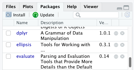
Додаткові пакети можна встановити із вкладки ‘packages’. На вкладці пакетів натисніть значок ‘Install’ (Встановити) і почніть вводити назву потрібного пакета у текстовому полі. Під час введення тексту пакети, назви яких починаються з введених вами символів, будуть показуватися у випадному списку і ви зможете вибрати потрібний.

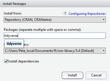
У нижній частині вікна Install Packages (Встановити пакети) є прапорець ‘Install’ dependencies (Встановити залежності). Цю опцію за замовчуванням увімкнено, і зазвичай саме так і потрібно. Пакети можуть (і справді) використовувати функціональність, вбудовану в інші пакети, тому для того, щоб функції пакета, який ви встановлюєте, працювали правильно, може знадобитися встановлення інших пакетів разом із ним. Опція ‘Install dependencies’ (встановити залежності) забезпечує, щоб ці додаткові пакети також були встановлені.

Challenge

Завдання

Використовуйте вкладку Console (Консоль) і Packages (Пакети), щоб переконатися, що у вас встановлено tidyverse.

Відповідь

Прокрутіть вкладку пакетів вниз до ‘tidyverse’. Ви також можете ввести кілька символів у вікно пошуку. Пакет ‘tidyverse’ насправді є набором пакетів, включаючи ‘ggplot2’ та ‘dplyr’, які обидва потребують інших пакетів для коректної роботи. Всі ці пакети будуть встановлені автоматично. Залежно від того, які пакети раніше були встановлені у вашому середовищі R, встановлення ‘tidyverse’ може бути дуже швидким або ж зайняти кілька хвилин. Під час встановлення на консолі будуть виводитися повідомлення, пов’язані з прогресом його виконання. Ви зможете побачити всі пакети, які фактично встановлюються.

Оскільки процес встановлення отримує доступ до сховища CRAN, вам знадобиться підключення до Інтернету для встановлення пакетів.

Також можна встановити пакети з інших репозиторіїв, в тому числі з Github або локальної файлової системи, але ми не будемо розглядати ці варіанти в цьому уроці.

Встановлення додаткових пакетів за допомогою команд R

---

Якщо ви дивилися вікно консолі під час запуску встановлення ‘tidyverse’, можливо, ви помітили, що рядок

R

install.packages("tidyverse")

був записаний на консоль до початку інсталяційних повідомлень.

Ви також могли встановити пакети tidyverse, виконавши цю команду безпосередньо в терміналі R.

Ми будемо використовувати ще один пакет під назвою here протягом усього курсу для керування шляхами та каталогами. Ми обговоримо це більш детально в пізньому епізоді, але зараз ми встановимо його в консолі:

R

install.packages("here")

Key Points

• Використовуйте RStudio для створення та запуску програм R.
• Використовуйте install.packages() для встановлення пакетів (бібліотек).

Content from Введення до R

---

Last updated on 2026-01-17 | Edit this page

Estimated time: 80 minutes

Instructor Note

• Основна мета - познайомити користувачів з різними об’єктами в R, від елементарних типів до створення власних об’єктів.
• Хоча цей розділ є базовим, будьте обережні, щоб не “загрузнути в деталях”, адже різноманіття типів і операцій може бути надто складним для новачків — особливо до того, як вони зрозуміють, як усе це вписується у їх власний “робочий процес”.

Overview

Questions

• Які типи даних доступні в R?
• Що таке об’єкт?
• Як можна присвоювати іменам об’єкти різних типів даних?
• Які арифметичні та логічні оператори можна використовувати?
• Як можна отримати підмножини з векторів?
• Як в R трактувати відсутні значення?
• Як ми можемо впоратися з відсутніми значеннями в R?

Objectives

• Визначити такі терміни, як вони стосуються R: об’єкт, призначення, виклик, функція, аргументи, параметри.
• Призначити значення іменам у R.
• Дізнатися, як називати об’єкти.
• Використовувати коментарі для інформування сценарію.
• Розв’язувати прості арифметичні операції в R.
• Викликати функції та використовувати аргументи, щоб змінити їх параметри за замовчуванням.
• Оглянути вміст векторів і маніпулювати їх вмістом.
• Значення підмножини з векторів.
• Аналізувати вектори з відсутніми даними.

Створення об’єктів в R

---

Ви можете використовувати R для простих математичних обчислень, друкуючи формули у консолі:

R

3 + 5

OUTPUT

[1] 8

R

12 / 7

OUTPUT

[1] 1.714286

Все, що існує в R - це об’єкти: від простих числових значень та рядків до складніших об’єктів, таких як вектори, матриці та списки. Навіть вирази й функції є об’єктами в R.

Однак, щоб робити корисні та цікаві речі, нам потрібно звертатися до об’єктів. Для цього нам потрібно вказати ім’я, за яким слідує оператор присвоєння <-, і об’єкт, який ми хочемо назвати:

R

areaHectares <- 1.0

<- - оператор присвоєння. Він призначає значення (об’єкти) праворуч іменам (також званим символами) на ліворуч. Отже, після виконання x <- 3 значення x дорівнює 3. Стрілку можна прочитати як 3 переходить в x. З історичних причин ви також можете використовувати = для присвоєння, але не в кожному контексті. Через незначні відмінності у синтаксисі, рекомендується завжди використовувати <- для присвоєння. Більше загалом ми віддаємо перевагу синтаксису <- перед =, оскільки він дає зрозуміти, в якому напрямку працює призначення (ліве призначення), і це збільшує читабельність коду.

У RStudio ввівши Alt + - (натискайте Alt одночасно з клавішею -) запише <- за допомогою лише однієї комбінації швидких клавіш у Windows. На Mac, те ж саме можна зробити, вводячи Option + - (натискайте Option одночасно з клавішею -).

Об’єктам можна дати будь-яку назву, наприклад x, current_temperature або subject_id. Ви хочете, щоб ваші назви об’єктів були явними й не надто довгими. Вони не можуть починатися з числа (2x не є дійсним, але x2 є). R чутливий до регістру (наприклад, age відрізняється від Age). Є деякі назви, які не можна використовувати, оскільки вони є назвами фундаментальних об’єктів у R (наприклад, if, else, for, див. тут для повного списку). Загалом, навіть якщо це дозволено, краще не використовувати їх (наприклад, c, T, mean, data, df, weights). Якщо ви сумніваєтесь, перевірте довідку, щоб побачити, чи ім’я вже використовується. Також краще уникати крапок (.) у назві об’єкта, як у my.dataset. Існує багато об’єктів в R з крапками в назвах з історичних причин, але оскільки точки мають особливе значення в R (для методів) та інших мовах програмування, краще уникати їх. Рекомендований стиль написання називається snake _case, що передбачає використання лише малих літер та цифр та розділення кожного слова підкресленням (наприклад, animal _weight, average _income). Також рекомендується використовувати іменники для назв об’єктів, а дієслова для назв функцій. Важливо бути послідовним у стилізації вашого коду (де ви розміщуєте пробіли, як ви називаєте об’єкти тощо). Використання послідовного стилю кодування робить ваш код зрозумілішим для читання для вас та ваших співробітників. У R три популярні посібники зі стилю: Google, Jean Fan’s та tidyverse. Tidyverse дуже вичерпний і спочатку може здатися приголомшливим. Ви можете встановити пакет lintr, щоб автоматично перевіряти на наявність проблем у стилі вашого коду.

Callout

Об’єкти проти змінних

Іменування об’єктів у R якось пов’язане з змінними у багатьох інших мовах програмування. У багатьох мовах програмування змінна має три аспекти: ім’я, місце розташування пам’яті та поточне значення, що зберігається в цьому місці. R абстракції з модифікованих місць пам’яті. У R ми маємо лише об’єкти, які можна назвати. Залежно від контексту name (of a object)і variable можуть мати різко різні значення. Однак у цьому уроці два слова використовуються як синоніми. Для отримання додаткової інформації див.: https://cran.r-project.org/doc/manuals/r-release/R-lang.html#Objects

При присвоюванні значення назви, R не друкує нічого. Ви можете змусити R надрукувати значення за допомогою дужок або ввівши назву об’єкта:

R

area_hectares <- 1.0    # не виводить нічого
(area_hectares <- 1.0)  # якщо взяти вираз у дужки — він надрукує значення `area_hectares`

OUTPUT

[1] 1

R

area_hectares           # друкує значення також, якщо просто ввести назву об’єкта

OUTPUT

[1] 1

Тепер, коли R має area_hectares в пам’яті, ми можемо робити з ним арифметичні операції. Наприклад, ми можемо захотіти перетворити цю площу на гектари (площа в акрах дорівнює 2,47 р. більше площі в гектарах):

R

2.47 * area_hectares

OUTPUT

[1] 2.47

Ми також можемо змінити значення, присвоєне імені, призначивши йому нове:

R

area_hectares <- 2.5
2.47 * area_hectares

OUTPUT

[1] 6.175

Це означає, що присвоєння значення одному імені не змінює значення інших імен. Наприклад, назвемо площу ділянки в акрах areaAcres:

R

area_acres <- 2.47 * area_hectares

потім змінити (перепризначити) area_hectares на 50.

R

area_hectares <- 50

Challenge

Завдання

Як ви думаєте, яке поточне значення area_acres? 123.5 або 6.175?

Рішення

The value of area_acres is still 6.175 because you have not re-run the line area_acres <- 2.47 * area_hectares since changing the value of area_hectares.

Comments

---

All programming languages allow the programmer to include comments in their code. Including comments to your code has many advantages: it helps you explain your reasoning and it forces you to be tidy. A commented code is also a great tool not only to your collaborators, but to your future self. Comments are the key to a reproducible analysis.

To do this in R we use the # character. Anything to the right of the # sign and up to the end of the line is treated as a comment and is ignored by R. You can start lines with comments or include them after any code on the line.

R

area_hectares <- 1.0      # land area in hectares
area_acres <- area_hectares * 2.47  # convert to acres
area_acres        # print land area in acres.

OUTPUT

[1] 2.47

RStudio makes it easy to comment or uncomment a paragraph: after selecting the lines you want to comment, press at the same time on your keyboard Ctrl + Shift + C. If you only want to comment out one line, you can put the cursor at any location of that line (i.e. no need to select the whole line), then press Ctrl + Shift + C.

Challenge

Exercise

Create two variables r_length and r_width and assign them values. It should be noted that, because length is a built-in R function, R Studio might add “()” after you type length and if you leave the parentheses you will get unexpected results. This is why you might see other programmers abbreviate common words. Create a third variable r_area and give it a value based on the current values of r_length and r_width. Show that changing the values of either r_length and r_width does not affect the value of r_area.

Show me the solution

R

r_length <- 2.5
r_width <- 3.2
r_area <- r_length * r_width
r_area

OUTPUT

[1] 8

R

# change the values of r_length and r_width
r_length <- 7.0
r_width <- 6.5
# the value of r_area isn't changed
r_area

OUTPUT

[1] 8

Functions and their arguments

Functions are “canned scripts” that automate more complicated sets of commands including operations assignments, etc. Many functions are predefined, or can be made available by importing R packages (more on that later). A function usually gets one or more inputs called arguments. Functions often (but not always) return a value. A typical example would be the function sqrt(). The input (the argument) must be a number, and the return value (in fact, the output) is the square root of that number. Executing a function (‘running it’) is called calling the function. An example of a function call is:

R

b <- sqrt(a)

Here, the value of a is given to the sqrt() function, the sqrt() function calculates the square root, and returns the value which is then assigned to the name b. This function is very simple, because it takes just one argument.

The return ‘value’ of a function need not be numerical (like that of sqrt()), and it also does not need to be a single item: it can be a set of things, or even a dataset. We’ll see that when we read data files into R.

Arguments can be anything, not only numbers or filenames, but also other objects. Exactly what each argument means differs per function, and must be looked up in the documentation (see below). Some functions take arguments which may either be specified by the user, or, if left out, take on a default value: these are called options. Options are typically used to alter the way the function operates, such as whether it ignores ‘bad values’, or what symbol to use in a plot. However, if you want something specific, you can specify a value of your choice which will be used instead of the default.

Let’s try a function that can take multiple arguments: round().

R

round(3.14159)

OUTPUT

[1] 3

Here, we’ve called round() with just one argument, 3.14159, and it has returned the value 3. That’s because the default is to round to the nearest whole number. If we want more digits we can see how to do that by getting information about the round function. We can use args(round) or look at the help for this function using ?round.

R

args(round)

OUTPUT

function (x, digits = 0, ...)
NULL

R

?round

We see that if we want a different number of digits, we can type digits=2 or however many we want.

R

round(3.14159, digits = 2)

OUTPUT

[1] 3.14

If you provide the arguments in the exact same order as they are defined you don’t have to name them:

R

round(3.14159, 2)

OUTPUT

[1] 3.14

And if you do name the arguments, you can switch their order:

R

round(digits = 2, x = 3.14159)

OUTPUT

[1] 3.14

It’s good practice to put the non-optional arguments (like the number you’re rounding) first in your function call, and to specify the names of all optional arguments. If you don’t, someone reading your code might have to look up the definition of a function with unfamiliar arguments to understand what you’re doing.

Discussion

Exercise

Type in ?round at the console and then look at the output in the Help pane. What other functions exist that are similar to round? How do you use the digits parameter in the round function?

Vectors and data types

---

A vector is the most common and basic data type in R, and is pretty much the workhorse of R. A vector is composed by a series of values, which can be either numbers or characters. We can assign a series of values to a vector using the c() function. For example we can create a vector of the number of household members for the households we’ve interviewed and assign it to hh_members:

R

hh_members <- c(3, 7, 10, 6)
hh_members

OUTPUT

[1]  3  7 10  6

A vector can also contain characters. For example, we can have a vector of the building material used to construct our interview respondents’ walls (respondent_wall_type):

R

respondent_wall_type <- c("muddaub", "burntbricks", "sunbricks")
respondent_wall_type

OUTPUT

[1] "muddaub"     "burntbricks" "sunbricks"  

The quotes around “muddaub”, etc. are essential here. Without the quotes R will assume there are objects called muddaub, burntbricks and sunbricks. As these names don’t exist in R’s memory, there will be an error message.

There are many functions that allow you to inspect the content of a vector. length() tells you how many elements are in a particular vector:

R

length(hh_members)

OUTPUT

[1] 4

R

length(respondent_wall_type)

OUTPUT

[1] 3

An important feature of a vector, is that all of the elements are the same type of data. The function typeof() indicates the type of an object:

R

typeof(hh_members)

OUTPUT

[1] "double"

R

typeof(respondent_wall_type)

OUTPUT

[1] "character"

The function str() provides an overview of the structure of an object and its elements. It is a useful function when working with large and complex objects:

R

str(hh_members)

OUTPUT

 num [1:4] 3 7 10 6

R

str(respondent_wall_type)

OUTPUT

 chr [1:3] "muddaub" "burntbricks" "sunbricks"

You can use the c() function to add other elements to your vector:

R

possessions <- c("bicycle", "radio", "television")
possessions <- c(possessions, "mobile_phone") # add to the end of the vector
possessions <- c("car", possessions) # add to the beginning of the vector
possessions

OUTPUT

[1] "car"          "bicycle"      "radio"        "television"   "mobile_phone"

In the first line, we take the original vector possessions, add the value "mobile_phone" to the end of it, and save the result back into possessions. Then we add the value "car" to the beginning, again saving the result back into possessions.

We can do this over and over again to grow a vector, or assemble a dataset. As we program, this may be useful to add results that we are collecting or calculating.

An atomic vector is the simplest R data type and is a linear vector of a single type. Above, we saw 2 of the 6 main atomic vector types that R uses: "character" and "numeric" (or "double"). These are the basic building blocks that all R objects are built from. The other 4 atomic vector types are:

• "logical" for TRUE and FALSE (the boolean data type)
• "integer" for integer numbers (e.g., 2L, the L indicates to R that it’s an integer)
• "complex" to represent complex numbers with real and imaginary parts (e.g., 1 + 4i) and that’s all we’re going to say about them
• "raw" for bitstreams that we won’t discuss further

You can check the type of your vector using the typeof() function and inputting your vector as the argument.

Vectors are one of the many data structures that R uses. Other important ones are lists (list), matrices (matrix), data frames (data.frame), factors (factor) and arrays (array).

Challenge

Exercise

We’ve seen that atomic vectors can be of type character, numeric (or double), integer, and logical. But what happens if we try to mix these types in a single vector?

Show me the solution

R implicitly converts them to all be the same type.

Challenge

Exercise (continued)

What will happen in each of these examples? (hint: use class() to check the data type of your objects):

R

num_char <- c(1, 2, 3, "a")
num_logical <- c(1, 2, 3, TRUE)
char_logical <- c("a", "b", "c", TRUE)
tricky <- c(1, 2, 3, "4")

Why do you think it happens?

Show me the solution

Vectors can be of only one data type. R tries to convert (coerce) the content of this vector to find a “common denominator” that doesn’t lose any information.

Challenge

Exercise (continued)

How many values in combined_logical are "TRUE" (as a character) in the following example:

R

num_logical <- c(1, 2, 3, TRUE)
char_logical <- c("a", "b", "c", TRUE)
combined_logical <- c(num_logical, char_logical)

Show me the solution

Only one. There is no memory of past data types, and the coercion happens the first time the vector is evaluated. Therefore, the TRUE in num_logical gets converted into a 1 before it gets converted into "1" in combined_logical.

Discussion

Exercise (continued)

You’ve probably noticed that objects of different types get converted into a single, shared type within a vector. In R, we call converting objects from one class into another class coercion. These conversions happen according to a hierarchy, whereby some types get preferentially coerced into other types. Can you draw a diagram that represents the hierarchy of how these data types are coerced?

Subsetting vectors

---

Subsetting (sometimes referred to as extracting or indexing) involves accessing out one or more values based on their numeric placement or “index” within a vector. If we want to subset one or several values from a vector, we must provide one index or several indices in square brackets. For instance:

R

respondent_wall_type <- c("muddaub", "burntbricks", "sunbricks")
respondent_wall_type[2]

OUTPUT

[1] "burntbricks"

R

respondent_wall_type[c(3, 2)]

OUTPUT

[1] "sunbricks"   "burntbricks"

We can also repeat the indices to create an object with more elements than the original one:

R

more_respondent_wall_type <- respondent_wall_type[c(1, 2, 3, 2, 1, 3)]
more_respondent_wall_type

OUTPUT

[1] "muddaub"     "burntbricks" "sunbricks"   "burntbricks" "muddaub"
[6] "sunbricks"  

R indices start at 1. Programming languages like Fortran, MATLAB, Julia, and R start counting at 1, because that’s what human beings typically do. Languages in the C family (including C++, Java, Perl, and Python) count from 0 because that’s simpler for computers to do.

Conditional subsetting

Another common way of subsetting is by using a logical vector. TRUE will select the element with the same index, while FALSE will not:

R

hh_members <- c(3, 7, 10, 6)
hh_members[c(TRUE, FALSE, TRUE, TRUE)]

OUTPUT

[1]  3 10  6

Typically, these logical vectors are not typed by hand, but are the output of other functions or logical tests. For instance, if you wanted to select only the values above 5:

R

hh_members > 5    # will return logicals with TRUE for the indices that meet the condition

OUTPUT

[1] FALSE  TRUE  TRUE  TRUE

R

## so we can use this to select only the values above 5
hh_members[hh_members > 5]

OUTPUT

[1]  7 10  6

You can combine multiple tests using & (both conditions are true, AND) or | (at least one of the conditions is true, OR):

R

hh_members[hh_members < 4 | hh_members > 7]

OUTPUT

[1]  3 10

R

hh_members[hh_members >= 4 & hh_members <= 7]

OUTPUT

[1] 7 6

Here, < stands for “less than”, > for “greater than”, >= for “greater than or equal to”, and == for “equal to”. The double equal sign == is a test for numerical equality between the left and right hand sides, and should not be confused with the single = sign, which performs variable assignment (similar to <-).

A common task is to search for certain strings in a vector. One could use the “or” operator | to test for equality to multiple values, but this can quickly become tedious.

R

possessions <- c("car", "bicycle", "radio", "television", "mobile_phone")
possessions[possessions == "car" | possessions == "bicycle"] # returns both car and bicycle

OUTPUT

[1] "car"     "bicycle"

The function %in% allows you to test if any of the elements of a search vector (on the left hand side) are found in the target vector (on the right hand side):

R

possessions %in% c("car", "bicycle")

OUTPUT

[1]  TRUE  TRUE FALSE FALSE FALSE

Note that the output is the same length as the search vector on the left hand side, because %in% checks whether each element of the search vector is found somewhere in the target vector. Thus, you can use %in% to select the elements in the search vector that appear in your target vector:

R

possessions %in% c("car", "bicycle", "motorcycle", "truck", "boat", "bus")

OUTPUT

[1]  TRUE  TRUE FALSE FALSE FALSE

R

possessions[possessions %in% c("car", "bicycle", "motorcycle", "truck", "boat", "bus")]

OUTPUT

[1] "car"     "bicycle"

Missing data

---

As R was designed to analyze datasets, it includes the concept of missing data (which is uncommon in other programming languages). Missing data are represented in vectors as NA.

When doing operations on numbers, most functions will return NA if the data you are working with include missing values. This feature makes it harder to overlook the cases where you are dealing with missing data. You can add the argument na.rm=TRUE to calculate the result while ignoring the missing values.

R

rooms <- c(2, 1, 1, NA, 7)
mean(rooms)

OUTPUT

[1] NA

R

max(rooms)

OUTPUT

[1] NA

R

mean(rooms, na.rm = TRUE)

OUTPUT

[1] 2.75

R

max(rooms, na.rm = TRUE)

OUTPUT

[1] 7

If your data include missing values, you may want to become familiar with the functions is.na(), na.omit(), and complete.cases(). See below for examples.

R

## Extract those elements which are not missing values.
## The ! character is also called the NOT operator
rooms[!is.na(rooms)]

OUTPUT

[1] 2 1 1 7

R

## Count the number of missing values.
## The output of is.na() is a logical vector (TRUE/FALSE equivalent to 1/0) so the sum() function here is effectively counting
sum(is.na(rooms))

OUTPUT

[1] 1

R

## Returns the object with incomplete cases removed. The returned object is an atomic vector of type `"numeric"` (or `"double"`).
na.omit(rooms)

OUTPUT

[1] 2 1 1 7
attr(,"na.action")
[1] 4
attr(,"class")
[1] "omit"

R

## Extract those elements which are complete cases. The returned object is an atomic vector of type `"numeric"` (or `"double"`).
rooms[complete.cases(rooms)]

OUTPUT

[1] 2 1 1 7

Recall that you can use the typeof() function to find the type of your atomic vector.

Challenge

Exercise

1. Using this vector of rooms, create a new vector with the NAs removed.

R

rooms <- c(1, 2, 1, 1, NA, 3, 1, 3, 2, 1, 1, 8, 3, 1, NA, 1)

2. Use the function median() to calculate the median of the rooms vector.

3. Use R to figure out how many households in the set use more than 2 rooms for sleeping.

Show me the solution

R

rooms <- c(1, 2, 1, 1, NA, 3, 1, 3, 2, 1, 1, 8, 3, 1, NA, 1)
rooms_no_na <- rooms[!is.na(rooms)]
# or
rooms_no_na <- na.omit(rooms)
# 2.
median(rooms, na.rm = TRUE)

OUTPUT

[1] 1

R

# 3.
rooms_above_2 <- rooms_no_na[rooms_no_na > 2]
length(rooms_above_2)

OUTPUT

[1] 4

Now that we have learned how to write scripts, and the basics of R’s data structures, we are ready to start working with the SAFI dataset we have been using in the other lessons, and learn about data frames.

Key Points

• Access individual values by location using [].
• Access arbitrary sets of data using [c(...)].
• Use logical operations and logical vectors to access subsets of data.

Content from Починаємо з даних

---

Last updated on 2026-01-17 | Edit this page

Estimated time: 80 minutes

Instructor Note

Дві основні цілі цих уроків:

• Переконатися, що учасники впевнено працюють із датафреймом і можуть використовувати дужки для вибору рядків і стовпців.
• Виставити учнів як фактори. Їхня поведінка не завжди інтуїтивно зрозуміла, тому важливо, щоб учасників супроводжували під час роботи з ними вперше. The content of the lesson should be enough for learners to avoid common mistakes with them.

Overview

Questions

• Що таке датафрейм?
• Як я можу прочитати повний файл csv в R?
• Як я можу отримати основну зведену інформацію про мій набір даних?
• Як я можу змінити спосіб обробки R рядків у моєму наборі даних?
• Чому мені потрібно, щоб текстові рядки оброблялися інакше?
• Як у R представлені дати і як можна змінити їхній формат?

Objectives

• Описати що таке датафрейм.
• Завантажити зовнішні дані з файлу .csv в датафрейм.
• Підсумувати вміст датафрейму.
• Вибрати підмножину значень із датафреймів.
• Пояснити різницю між фактором і рядком.
• Перетворення між рядками та факторами.
• Упорядкувати та перейменувати фактори.
• Змінити спосіб обробки символьних рядків у датафреймі.
• Перевірити та змінити формат дат.

Що таке датафрейми?

---

Датафрейм - це стандартна структура даних для табличних даних у R, яку ми використовуємо для обробки даних, статистичного аналізу та візуалізації.

Датафрейм - це представлення даних у форматі таблиці, де стовпці є векторами, які мають однакову довжину. Датафрейми можна порівняти зі звичною електронною таблицею в програмах на кшталт Excel, але є одна важлива відмінність. Оскільки стовпці є векторами, кожен стовпець повинен містити один тип даних (наприклад, символи, цілі числа, фактори). Наприклад, на зображенні показано датафрейм, який складається з числового (numeric), текстового (character) та логічного (logical) векторів.

Датафрейм можна створювати вручну, але найчастіше вони генеруються функціями read_csv()або read_table(); іншими словами, при імпорті електронних таблиць з вашого жорсткого диска (або Інтернету). Тепер ми продемонструємо, як імпортувати табличні дані за допомогою read_csv().

Презентація даних SAFI

---

SAFI (Studying African Farmer-Led Irrigation) — це дослідження, яке вивчає методи ведення сільського господарства та іригації в Танзанії та Мозамбіку. Дані опитування були зібрані за допомогою інтерв’ю, проведених у період з листопада 2016 року до червня 2017 року. Для цього уроку ми будемо використовувати підмножину доступних даних. Для отримання інформації про повний навчальний набір даних, який використовується в інших уроках цього семінару, дивіться опис набору даних.

Ми будемо використовувати підмножину очищеної версії набору даних, яку було створено шляхом очищення в OpenRefine (data/SAFI_clean.csv). У цьому наборі даних відсутні значення позначені як “NULL”, кожен рядок містить інформацію про одного респондента інтерв’ю, а стовпці представляють:

назва/стовпця	опис
key_id	Додано, щоб надати унікальний ідентифікатор для кожного спостереження. (Поле InstanceID також робить це, але воно не так зручно у використанні)
village	Назва села
interview_date	Дата співбесіди
no_membrs	Скільки членів у домогосподарстві?
years_liv	Скільки років ви живете в цьому селі чи сусідньому селі?
respondent_wall_type	Який тип стін має їхній будинок (зі списку)
rooms	Скільки кімнат в основному будинку використовується для сну?
memb_assoc	Ви член зрошувальної асоціації?
affect_conflicts	Ви постраждали від конфліктів з іншими іригаторами в цьому районі?
liv_count	Кількість тваринництва, що перебуває у власності.
items_owned	Які з перерахованих предметів належать домогосподарству? (список)
no_meals	Скільки страв люди у вашому домогосподарстві зазвичай їдять за день?
months_lack_food	Вкажіть, на які місяці, в останні 12 місяців ви стикалися з ситуацією, коли у вас не було достатньо їжі, щоб прогодувати домогосподарство?
instanceID	Унікальний ідентифікатор для подання даних форми

Імпорт даних

---

Ви збираєтеся завантажити дані в пам’ять R за допомогою функції read_csv() з пакета readr, який є частиною tidyverse; дізнайтеся більше про колекцію пакетів tidyverse тут. readr встановлюється як частина tidyverse встановлення. Коли ви завантажуєте tidyverse (library(tidyverse)), завантажуються основні пакети (пакети, які використовуються в більшості аналізів даних), включаючи readr.

Однак, перш ніж продовжити, це хороша можливість поговорити про конфлікти. Деякі пакети, які ми завантажуємо, можуть в кінцевому підсумку вводити імена функцій, які вже використовуються попередньо завантаженими пакетами R. Наприклад, коли ми завантажимо пакет tidyverse нижче, ми введемо дві суперечливі функції: filter()і lag(). Це відбувається тому, що filter і lag вже є функціями, які використовуються пакетом stats (вже попередньо завантажений у R). Тепер, якщо ми, наприклад, викликаємо функцію filter(), R використовуватиме dplyr::filter() версії, а не stats::filter(). Це відбувається тому, що, якщо це конфлікт, за замовчуванням R використовує функцію з останнього завантаженого пакета. Конфліктні функції можуть викликати у вас певні проблеми в майбутньому, тому важливо, щоб ми знали про них, щоб ми могли правильно обробляти їх, якщо хочемо.

To do so, we just need the following functions from the conflicted package:

• conflicted::conflict_scout(): Shows us any conflicted functions.
• conflict_prefer("function", "package_prefered"): Allows us to choose the default function we want from now on.

It is also important to know that we can, at any time, just call the function directly from the package we want, such as stats::filter().

Even with the use of an RStudio project, it can be difficult to learn how to specify paths to file locations. Enter the here package! The here package creates paths relative to the top-level directory (your RStudio project). These relative paths work regardless of where the associated source file lives inside your project, like analysis projects with data and reports in different subdirectories. This is an important contrast to using setwd(), which depends on the way you order your files on your computer.

Image credit: Allison Horst

Before we can use the read_csv() and here() functions, we need to load the tidyverse and here packages.

Also, if you recall, the missing data is encoded as “NULL” in the dataset. We’ll tell it to the function, so R will automatically convert all the “NULL” entries in the dataset into NA.

R

library(tidyverse)
library(here)

interviews <- read_csv(
  here("data", "SAFI_clean.csv"), 
  na = "NULL")

In the above code, we notice the here() function takes folder and file names as inputs (e.g., "data", "SAFI_clean.csv"), each enclosed in quotations ("") and separated by a comma. The here() will accept as many names as are necessary to navigate to a particular file (e.g., here("analysis", "data", "surveys", "clean", "SAFI_clean.csv)).

The here() function can accept the folder and file names in an alternate format, using a slash (“/”) rather than commas to separate the names. The two methods are equivalent, so that here("data", "SAFI_clean.csv") and here("data/SAFI_clean.csv") produce the same result. (The slash is used on all operating systems; backslashes are not used.)

If you were to type in the code above, it is likely that the read.csv() function would appear in the automatically populated list of functions. This function is different from the read_csv() function, as it is included in the “base” packages that come pre-installed with R. Overall, read.csv() behaves similar to read_csv(), with a few notable differences. First, read.csv() coerces column names with spaces and/or special characters to different names (e.g. interview date becomes interview.date). Second, read.csv() stores data as a data.frame, where read_csv() stores data as a different kind of data frame called a tibble. We prefer tibbles because they have nice printing properties among other desirable qualities. Read more about tibbles here.

The second statement in the code above creates a data frame but doesn’t output any data because, as you might recall, assignments (<-) don’t display anything. (Note, however, that read_csv may show informational text about the data frame that is created.) If we want to check that our data has been loaded, we can see the contents of the data frame by typing its name: interviews in the console.

R

interviews
## Try also
## view(interviews)
## head(interviews)

OUTPUT

# A tibble: 131 × 14
   key_ID village  interview_date      no_membrs years_liv respondent_wall_type
    <dbl> <chr>    <dttm>                  <dbl>     <dbl> <chr>
 1      1 God      2016-11-17 00:00:00         3         4 muddaub
 2      2 God      2016-11-17 00:00:00         7         9 muddaub
 3      3 God      2016-11-17 00:00:00        10        15 burntbricks
 4      4 God      2016-11-17 00:00:00         7         6 burntbricks
 5      5 God      2016-11-17 00:00:00         7        40 burntbricks
 6      6 God      2016-11-17 00:00:00         3         3 muddaub
 7      7 God      2016-11-17 00:00:00         6        38 muddaub
 8      8 Chirodzo 2016-11-16 00:00:00        12        70 burntbricks
 9      9 Chirodzo 2016-11-16 00:00:00         8         6 burntbricks
10     10 Chirodzo 2016-12-16 00:00:00        12        23 burntbricks
# ℹ 121 more rows
# ℹ 8 more variables: rooms <dbl>, memb_assoc <chr>, affect_conflicts <chr>,
#   liv_count <dbl>, items_owned <chr>, no_meals <dbl>, months_lack_food <chr>,
#   instanceID <chr>

Callout

Note

read_csv() assumes that fields are delimited by commas. However, in several countries, the comma is used as a decimal separator and the semicolon (;) is used as a field delimiter. If you want to read in this type of files in R, you can use the read_csv2 function. It behaves exactly like read_csv but uses different parameters for the decimal and the field separators. If you are working with another format, they can be both specified by the user. Check out the help for read_csv() by typing ?read_csv to learn more. There is also the read_tsv() for tab-separated data files, and read_delim() allows you to specify more details about the structure of your file.

Note that read_csv() actually loads the data as a tibble. A tibble is an extension of R data frames used by the tidyverse. When the data is read using read_csv(), it is stored in an object of class tbl_df, tbl, and data.frame. You can see the class of an object with

R

class(interviews)

OUTPUT

[1] "spec_tbl_df" "tbl_df"      "tbl"         "data.frame" 

As a tibble, the type of data included in each column is listed in an abbreviated fashion below the column names. For instance, here key_ID is a column of floating point numbers (abbreviated <dbl> for the word ‘double’), village is a column of characters (<chr>) and the interview_date is a column in the “date and time” format (<dttm>).

Inspecting data frames

---

When calling a tbl_df object (like interviews here), there is already a lot of information about our data frame being displayed such as the number of rows, the number of columns, the names of the columns, and as we just saw the class of data stored in each column. However, there are functions to extract this information from data frames. Here is a non-exhaustive list of some of these functions. Let’s try them out!

Size:

• dim(interviews) - returns a vector with the number of rows as the first element, and the number of columns as the second element (the dimensions of the object)
• nrow(interviews)- повертає кількість рядків
• ncol(interviews) - повертає кількість стовпців

Content:

• head(interviews) - shows the first 6 rows
• tail(interviews) - shows the last 6 rows

Names:

• names(interviews) - returns the column names (synonym of colnames() for data.frame objects)

Summary:

• str(interviews) - structure of the object and information about the class, length and content of each column
• summary(interviews) - summary statistics for each column
• glimpse(interviews) - returns the number of columns and rows of the tibble, the names and class of each column, and previews as many values will fit on the screen. Unlike the other inspecting functions listed above, glimpse() is not a “base R” function so you need to have the dplyr or tibble packages loaded to be able to execute it.

Note: most of these functions are “generic.” They can be used on other types of objects besides data frames or tibbles.

Subsetting data frames

---

Our interviews data frame has rows and columns (it has 2 dimensions). In practice, we may not need the entire data frame; for instance, we may only be interested in a subset of the observations (the rows) or a particular set of variables (the columns). If we want to access some specific data from it, we need to specify the “coordinates” (i.e., indices) we want from it. Row numbers come first, followed by column numbers.

Callout

Tip

Subsetting a tibble with [ always results in a tibble. However, note this is not true in general for data frames, so be careful! Different ways of specifying these coordinates can lead to results with different classes. This is covered in the Software Carpentry lesson R for Reproducible Scientific Analysis.

R

## first element in the first column of the tibble
interviews[1, 1]

OUTPUT

# A tibble: 1 × 1
  key_ID
   <dbl>
1      1

R

## first element in the 6th column of the tibble 
interviews[1, 6]

OUTPUT

# A tibble: 1 × 1
  respondent_wall_type
  <chr>
1 muddaub             

R

## first column of the tibble (as a vector)
interviews[[1]]

OUTPUT

  [1]   1   2   3   4   5   6   7   8   9  10  11  12  13  14  15  16  17  18
 [19]  19  20  21  22  23  24  25  26  27  28  29  30  31  32  33  34  35  36
 [37]  37  38  39  40  41  42  43  44  45  46  47  48  49  50  51  52  53  54
 [55]  55  56  57  58  59  60  61  62  63  64  65  66  67  68  69  70  71 127
 [73] 133 152 153 155 178 177 180 181 182 186 187 195 196 197 198 201 202  72
 [91]  73  76  83  85  89 101 103 102  78  80 104 105 106 109 110 113 118 125
[109] 119 115 108 116 117 144 143 150 159 160 165 166 167 174 175 189 191 192
[127] 126 193 194 199 200

R

## first column of the tibble
interviews[1]

OUTPUT

# A tibble: 131 × 1
   key_ID
    <dbl>
 1      1
 2      2
 3      3
 4      4
 5      5
 6      6
 7      7
 8      8
 9      9
10     10
# ℹ 121 more rows

R

## first three elements in the 7th column of the tibble
interviews[1:3, 7]

OUTPUT

# A tibble: 3 × 1
  rooms
  <dbl>
1     1
2     1
3     1

R

## the 3rd row of the tibble
interviews[3, ]

OUTPUT

# A tibble: 1 × 14
  key_ID village interview_date      no_membrs years_liv respondent_wall_type
   <dbl> <chr>   <dttm>                  <dbl>     <dbl> <chr>
1      3 God     2016-11-17 00:00:00        10        15 burntbricks
# ℹ 8 more variables: rooms <dbl>, memb_assoc <chr>, affect_conflicts <chr>,
#   liv_count <dbl>, items_owned <chr>, no_meals <dbl>, months_lack_food <chr>,
#   instanceID <chr>

R

## equivalent to head_interviews <- head(interviews)
head_interviews <- interviews[1:6, ]

: is a special function that creates numeric vectors of integers in increasing or decreasing order, test 1:10 and 10:1 for instance.

You can also exclude certain indices of a data frame using the “-” sign:

R

interviews[, -1]          # The whole tibble, except the first column

OUTPUT

# A tibble: 131 × 13
   village  interview_date      no_membrs years_liv respondent_wall_type rooms
   <chr>    <dttm>                  <dbl>     <dbl> <chr>                <dbl>
 1 God      2016-11-17 00:00:00         3         4 muddaub                  1
 2 God      2016-11-17 00:00:00         7         9 muddaub                  1
 3 God      2016-11-17 00:00:00        10        15 burntbricks              1
 4 God      2016-11-17 00:00:00         7         6 burntbricks              1
 5 God      2016-11-17 00:00:00         7        40 burntbricks              1
 6 God      2016-11-17 00:00:00         3         3 muddaub                  1
 7 God      2016-11-17 00:00:00         6        38 muddaub                  1
 8 Chirodzo 2016-11-16 00:00:00        12        70 burntbricks              3
 9 Chirodzo 2016-11-16 00:00:00         8         6 burntbricks              1
10 Chirodzo 2016-12-16 00:00:00        12        23 burntbricks              5
# ℹ 121 more rows
# ℹ 7 more variables: memb_assoc <chr>, affect_conflicts <chr>,
#   liv_count <dbl>, items_owned <chr>, no_meals <dbl>, months_lack_food <chr>,
#   instanceID <chr>

R

interviews[-c(7:131), ]   # Equivalent to head(interviews)

OUTPUT

# A tibble: 6 × 14
  key_ID village interview_date      no_membrs years_liv respondent_wall_type
   <dbl> <chr>   <dttm>                  <dbl>     <dbl> <chr>
1      1 God     2016-11-17 00:00:00         3         4 muddaub
2      2 God     2016-11-17 00:00:00         7         9 muddaub
3      3 God     2016-11-17 00:00:00        10        15 burntbricks
4      4 God     2016-11-17 00:00:00         7         6 burntbricks
5      5 God     2016-11-17 00:00:00         7        40 burntbricks
6      6 God     2016-11-17 00:00:00         3         3 muddaub
# ℹ 8 more variables: rooms <dbl>, memb_assoc <chr>, affect_conflicts <chr>,
#   liv_count <dbl>, items_owned <chr>, no_meals <dbl>, months_lack_food <chr>,
#   instanceID <chr>

tibbles can be subset by calling indices (as shown previously), but also by calling their column names directly:

R

interviews["village"]       # Result is a tibble

interviews[, "village"]     # Result is a tibble

interviews[["village"]]     # Result is a vector

interviews$village          # Result is a vector

In RStudio, you can use the autocompletion feature to get the full and correct names of the columns.

Challenge

Завдання

1. Create a tibble (interviews_100) containing only the data in row 100 of the interviews dataset.

Now, continue using interviews for each of the following activities:

2. Notice how nrow() gave you the number of rows in the tibble?

• Use that number to pull out just that last row in the tibble.
• Compare that with what you see as the last row using tail() to make sure it’s meeting expectations.
• Pull out that last row using nrow() instead of the row number.
• Create a new tibble (interviews_last) from that last row.

3. Using the number of rows in the interviews dataset that you found in question 2, extract the row that is in the middle of the dataset. Store the content of this middle row in an object named interviews_middle. (hint: This dataset has an odd number of rows, so finding the middle is a bit trickier than dividing n_rows by 2. Use the median( ) function and what you’ve learned about sequences in R to extract the middle row!

4. Combine nrow() with the - notation above to reproduce the behavior of head(interviews), keeping just the first through 6th rows of the interviews dataset.

Відповідь

R

## 1.
interviews_100 <- interviews[100, ]
## 2.
# Saving `n_rows` to improve readability and reduce duplication
n_rows <- nrow(interviews)
interviews_last <- interviews[n_rows, ]
## 3.
interviews_middle <- interviews[median(1:n_rows), ]
## 4.
interviews_head <- interviews[-(7:n_rows), ]

Фактори

---

R has a special data class, called factor, to deal with categorical data that you may encounter when creating plots or doing statistical analyses. Factors are very useful and actually contribute to making R particularly well suited to working with data. So we are going to spend a little time introducing them.

Factors represent categorical data. They are stored as integers associated with labels and they can be ordered (ordinal) or unordered (nominal). Factors create a structured relation between the different levels (values) of a categorical variable, such as days of the week or responses to a question in a survey. This can make it easier to see how one element relates to the other elements in a column. While factors look (and often behave) like character vectors, they are actually treated as integer vectors by R. So you need to be very careful when treating them as strings.

Once created, factors can only contain a pre-defined set of values, known as levels. By default, R always sorts levels in alphabetical order. For instance, if you have a factor with 2 levels:

R

respondent_floor_type <- factor(c("earth", "cement", "cement", "earth"))

R will assign 1 to the level "cement" and 2 to the level "earth" (because c comes before e, even though the first element in this vector is "earth"). You can see this by using the function levels() and you can find the number of levels using nlevels():

R

levels(respondent_floor_type)

OUTPUT

[1] "cement" "earth" 

R

nlevels(respondent_floor_type)

OUTPUT

[1] 2

Sometimes, the order of the factors does not matter. Other times you might want to specify the order because it is meaningful (e.g., “low”, “medium”, “high”). It may improve your visualization, or it may be required by a particular type of analysis. Here, one way to reorder our levels in the respondent_floor_type vector would be:

R

respondent_floor_type # current order

OUTPUT

[1] earth  cement cement earth
Levels: cement earth

R

respondent_floor_type <- factor(respondent_floor_type, 
                                levels = c("earth", "cement"))

respondent_floor_type # after re-ordering

OUTPUT

[1] earth  cement cement earth
Levels: earth cement

In R’s memory, these factors are represented by integers (1, 2), but are more informative than integers because factors are self describing: "cement", "earth" is more descriptive than 1, and 2. Which one is “earth”? You wouldn’t be able to tell just from the integer data. Factors, on the other hand, have this information built in. It is particularly helpful when there are many levels. It also makes renaming levels easier. Let’s say we made a mistake and need to recode “cement” to “brick”. We can do this using the fct_recode() function from the forcats package (included in the tidyverse) which provides some extra tools to work with factors.

R

levels(respondent_floor_type)

OUTPUT

[1] "earth"  "cement"

R

respondent_floor_type <- fct_recode(respondent_floor_type, brick = "cement")

## as an alternative, we could change the "cement" level directly using the
## levels() function, but we have to remember that "cement" is the second level
# levels(respondent_floor_type)[2] <- "brick"

levels(respondent_floor_type)

OUTPUT

[1] "earth" "brick"

R

respondent_floor_type

OUTPUT

[1] earth brick brick earth
Levels: earth brick

So far, your factor is unordered, like a nominal variable. R does not know the difference between a nominal and an ordinal variable. You make your factor an ordered factor by using the ordered=TRUE option inside your factor function. Note how the reported levels changed from the unordered factor above to the ordered version below. Ordered levels use the less than sign < to denote level ranking.

R

respondent_floor_type_ordered <- factor(respondent_floor_type, 
                                        ordered = TRUE)

respondent_floor_type_ordered # after setting as ordered factor

OUTPUT

[1] earth brick brick earth
Levels: earth < brick

Converting factors

If you need to convert a factor to a character vector, you use as.character(x).

R

as.character(respondent_floor_type)

OUTPUT

[1] "earth" "brick" "brick" "earth"

Converting factors where the levels appear as numbers (such as concentration levels, or years) to a numeric vector is a little trickier. The as.numeric() function returns the index values of the factor, not its levels, so it will result in an entirely new (and unwanted in this case) set of numbers. One method to avoid this is to convert factors to characters, and then to numbers. Another method is to use the levels() function. Compare:

R

year_fct <- factor(c(1990, 1983, 1977, 1998, 1990))

as.numeric(year_fct)                     # Wrong! And there is no warning...

OUTPUT

[1] 3 2 1 4 3

R

as.numeric(as.character(year_fct))       # Works...

OUTPUT

[1] 1990 1983 1977 1998 1990

R

as.numeric(levels(year_fct))[year_fct]   # The recommended way.

OUTPUT

[1] 1990 1983 1977 1998 1990

Notice that in the recommended levels() approach, three important steps occur:

• We obtain all the factor levels using levels(year_fct)
• We convert these levels to numeric values using as.numeric(levels(year_fct))
• We then access these numeric values using the underlying integers of the vector year_fct inside the square brackets

Renaming factors

When your data is stored as a factor, you can use the plot() function to get a quick glance at the number of observations represented by each factor level. Let’s extract the memb_assoc column from our data frame, convert it into a factor, and use it to look at the number of interview respondents who were or were not members of an irrigation association:

R

## create a vector from the data frame column "memb_assoc"
memb_assoc <- interviews$memb_assoc

## convert it into a factor
memb_assoc <- as.factor(memb_assoc)

## let's see what it looks like
memb_assoc

OUTPUT

  [1] <NA> yes  <NA> <NA> <NA> <NA> no   yes  no   no   <NA> yes  no   <NA> yes
 [16] <NA> <NA> <NA> <NA> <NA> no   <NA> <NA> no   no   no   <NA> no   yes  <NA>
 [31] <NA> yes  no   yes  yes  yes  <NA> yes  <NA> yes  <NA> no   no   <NA> no
 [46] no   yes  <NA> <NA> yes  <NA> no   yes  no   <NA> yes  no   no   <NA> no
 [61] yes  <NA> <NA> <NA> no   yes  no   no   no   no   yes  <NA> no   yes  <NA>
 [76] <NA> yes  no   no   yes  no   no   yes  no   yes  no   no   <NA> yes  yes
 [91] yes  yes  yes  no   no   no   no   yes  no   no   yes  yes  no   <NA> no
[106] no   <NA> no   no   <NA> no   <NA> <NA> no   no   no   no   yes  no   no
[121] no   no   no   no   no   no   no   no   no   yes  <NA>
Levels: no yes

R

## bar plot of the number of interview respondents who were
## members of irrigation association:
plot(memb_assoc)

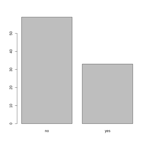
Looking at the plot compared to the output of the vector, we can see that in addition to “no”s and “yes”s, there are some respondents for whom the information about whether they were part of an irrigation association hasn’t been recorded, and encoded as missing data. These respondents do not appear on the plot. Let’s encode them differently so they can be counted and visualized in our plot.

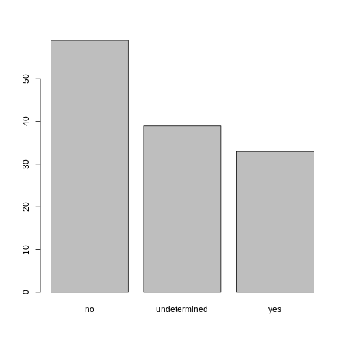
R

## Let's recreate the vector from the data frame column "memb_assoc"
memb_assoc <- interviews$memb_assoc

## replace the missing data with "undetermined"
memb_assoc[is.na(memb_assoc)] <- "undetermined"

## convert it into a factor
memb_assoc <- as.factor(memb_assoc)

## let's see what it looks like
memb_assoc

OUTPUT

  [1] undetermined yes          undetermined undetermined undetermined
  [6] undetermined no           yes          no           no
 [11] undetermined yes          no           undetermined yes
 [16] undetermined undetermined undetermined undetermined undetermined
 [21] no           undetermined undetermined no           no
 [26] no           undetermined no           yes          undetermined
 [31] undetermined yes          no           yes          yes
 [36] yes          undetermined yes          undetermined yes
 [41] undetermined no           no           undetermined no
 [46] no           yes          undetermined undetermined yes
 [51] undetermined no           yes          no           undetermined
 [56] yes          no           no           undetermined no
 [61] yes          undetermined undetermined undetermined no
 [66] yes          no           no           no           no
 [71] yes          undetermined no           yes          undetermined
 [76] undetermined yes          no           no           yes
 [81] no           no           yes          no           yes
 [86] no           no           undetermined yes          yes
 [91] yes          yes          yes          no           no
 [96] no           no           yes          no           no
[101] yes          yes          no           undetermined no
[106] no           undetermined no           no           undetermined
[111] no           undetermined undetermined no           no
[116] no           no           yes          no           no
[121] no           no           no           no           no
[126] no           no           no           no           yes
[131] undetermined
Levels: no undetermined yes

R

## bar plot of the number of interview respondents who were
## members of irrigation association:
plot(memb_assoc)

Challenge

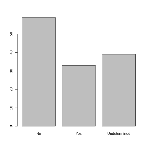
Завдання

• Rename the levels of the factor to have the first letter in uppercase: “No”,“Undetermined”, and “Yes”.

• Now that we have renamed the factor level to “Undetermined”, can you recreate the barplot such that “Undetermined” is last (after “Yes”)?

Відповідь

R

## Rename levels.
memb_assoc <- fct_recode(memb_assoc, No = "no",
                         Undetermined = "undetermined", Yes = "yes")
## Reorder levels. Note we need to use the new level names.
memb_assoc <- factor(memb_assoc, levels = c("No", "Yes", "Undetermined"))
plot(memb_assoc)

Formatting Dates

---

One of the most common issues that new (and experienced!) R users have is converting date and time information into a variable that is appropriate and usable during analyses. A best practice for dealing with date data is to ensure that each component of your date is available as a separate variable. In our dataset, we have a column interview_date which contains information about the year, month, and day that the interview was conducted. Let’s convert those dates into three separate columns.

R

str(interviews)

We are going to use the package lubridate, , which is included in the tidyverse installation and should be loaded by default. However, if we deal with older versions of tidyverse (2022 and ealier), we can manually load it by typing library(lubridate).

If necessary, start by loading the required package:

R

library(lubridate)

The lubridate function ymd() takes a vector representing year, month, and day, and converts it to a Date vector. Date is a class of data recognized by R as being a date and can be manipulated as such. The argument that the function requires is flexible, but, as a best practice, is a character vector formatted as “YYYY-MM-DD”.

Let’s extract our interview_date column and inspect the structure:

R

dates <- interviews$interview_date
str(dates)

OUTPUT

 POSIXct[1:131], format: "2016-11-17" "2016-11-17" "2016-11-17" "2016-11-17" "2016-11-17" ...

When we imported the data in R, read_csv() recognized that this column contained date information. We can now use the day(), month() and year() functions to extract this information from the date, and create new columns in our data frame to store it:

R

interviews$day <- day(dates)
interviews$month <- month(dates)
interviews$year <- year(dates)
interviews

OUTPUT

# A tibble: 131 × 17
   key_ID village  interview_date      no_membrs years_liv respondent_wall_type
    <dbl> <chr>    <dttm>                  <dbl>     <dbl> <chr>
 1      1 God      2016-11-17 00:00:00         3         4 muddaub
 2      2 God      2016-11-17 00:00:00         7         9 muddaub
 3      3 God      2016-11-17 00:00:00        10        15 burntbricks
 4      4 God      2016-11-17 00:00:00         7         6 burntbricks
 5      5 God      2016-11-17 00:00:00         7        40 burntbricks
 6      6 God      2016-11-17 00:00:00         3         3 muddaub
 7      7 God      2016-11-17 00:00:00         6        38 muddaub
 8      8 Chirodzo 2016-11-16 00:00:00        12        70 burntbricks
 9      9 Chirodzo 2016-11-16 00:00:00         8         6 burntbricks
10     10 Chirodzo 2016-12-16 00:00:00        12        23 burntbricks
# ℹ 121 more rows
# ℹ 11 more variables: rooms <dbl>, memb_assoc <chr>, affect_conflicts <chr>,
#   liv_count <dbl>, items_owned <chr>, no_meals <dbl>, months_lack_food <chr>,
#   instanceID <chr>, day <int>, month <dbl>, year <dbl>

Зверніть увагу на три нові стовпці в кінці нашого датафрейму.

In our example above, the interview_date column was read in correctly as a Date variable but generally that is not the case. Date columns are often read in as character variables and one can use the as_date() function to convert them to the appropriate Date/POSIXctformat.

Припустимо, у нас є вектор дат у символьному форматі:

R

char_dates <- c("7/31/2012", "8/9/2014", "4/30/2016")
str(char_dates)

OUTPUT

 chr [1:3] "7/31/2012" "8/9/2014" "4/30/2016"

We can convert this vector to dates as :

R

as_date(char_dates, format = "%m/%d/%Y")

OUTPUT

[1] "2012-07-31" "2014-08-09" "2016-04-30"

Argument format tells the function the order to parse the characters and identify the month, day and year. Формат вище - це еквівалент мм/дд/рррр. Неправильний формат може призвести до помилок або неправильних результатів.

For example, observe what happens when we use a lower case y instead of upper case Y for the year.

R

as_date(char_dates, format = "%m/%d/%y")

WARNING

Warning: 3 failed to parse.

OUTPUT

[1] NA NA NA

Here, the %y part of the format stands for a two-digit year instead of a four-digit year, and this leads to parsing errors.

Or in the following example, observe what happens when the month and day elements of the format are switched.

R

as_date(char_dates, format = "%d/%m/%y")

WARNING

Warning: 3 failed to parse.

OUTPUT

[1] NA NA NA

Since there is no month numbered 30 or 31, the first and third dates cannot be parsed.

We can also use functions ymd(), mdy() or dmy() to convert character variables to date.

R

mdy(char_dates)

OUTPUT

[1] "2012-07-31" "2014-08-09" "2016-04-30"

Key Points

• Використовуйте read_csv для читання табличних даних у R.
• Використовуйте фактори для представлення категоріальних даних у R.

Content from Маніпулювання даними за допомогою пакету dplyr

---

Last updated on 2026-01-19 | Edit this page

Estimated time: 40 minutes

Instructor Note

• Цей урок буде зрозумілішим, якщо використовувати графіки, які наочно демонструють роботу команд dplyr. Ви можете змінити цю презентацію Google Slides та використати для свого семінару.
• Для цього уроку переконайтеся, що учні впевнено користуються оператором pipe (%>%).
• Також іноді виникає деяка плутанина щодо того, якими мають бути аргументи group_by , а також коли використовувати filter () та select ().

Overview

Questions

• Як вибрати певні рядки та/або стовпці з датафрейму?
• Як об’єднати кілька команд в одну команду?
• Як створювати нові стовпці або видаляти наявні стовпці з датафрейму?

Objectives

• Опишіть призначення пакета R та пакету dplyr.
• Виділіть певні стовпці в датасеті за допомогою функції dplyr select.
• Виберіть певні рядки в датасеті відповідно до умов фільтрації за допомогою функції dplyr filter.
• З’єднайте результат однієї з dplyr функції з введенням іншої функції з оператором ‘pipe’ %>%.
• Додайте нові стовпці дата сету які є функціями наявних стовпців з mutate.
• Використовуйте концепцію розділення-застосування-комбінування для аналізу даних.
• Використовуйте summarize, group_by та count, щоб розділити набір даних на групи спостережень, застосувати зведену статистику для кожної групи, а потім об’єднати результати.

dplyr — це пакет, який спрощує роботу з табличними даними, використовуючи обмежений набір функцій, що можна поєднувати для отримання та узагальнення інформації з ваших даних.

Як і readr, dplyr є частиною набору пакетів tidyverse. Ці пакети були завантажені в пам’ять R, коли ми раніше викликали library (tidyverse).

Callout

Примітка

The packages in the tidyverse, namely dplyr, tidyr and ggplot2 accept both the British (e.g. summarise) and American (e.g. summarize) spelling variants of different function and option names. For this lesson, we utilize the American spellings of different functions; however, feel free to use the regional variant for where you are teaching.

What is an R package?

---

The package dplyr provides easy tools for the most common data wrangling tasks. It is built to work directly with dataframes, with many common tasks optimized by being written in a compiled language (C++) (not all R packages are written in R!).

There are also packages available for a wide range of tasks including building plots (ggplot2, which we’ll see later), downloading data from the NCBI database, or performing statistical analysis on your data set. Many packages such as these are housed on, and downloadable from, the Comprehensive R Archive Network (CRAN) using install.packages. This function makes the package accessible by your R installation with the command library(), as you did with tidyverse earlier.

To easily access the documentation for a package within R or RStudio, use help(package = "package_name").

To learn more about dplyr after the workshop, you may want to check out this handy data transformation with dplyr cheatsheet.

Callout

Примітка

There are alternatives to the tidyverse packages for data wrangling, including the package data.table. See this comparison for example to get a sense of the differences between using base, tidyverse, and data.table.

Вивчення dplyr

---

To make sure everyone will use the same dataset for this lesson, we’ll read again the SAFI dataset that we downloaded earlier.

R

## load the tidyverse
library(tidyverse)
library(here)

interviews <- read_csv(here("data", "SAFI_clean.csv"), na = "NULL")

## inspect the data
interviews

## preview the data
# view(interviews)

Ми вивчимо деякі з найпоширеніших функцій dplyr:

• select(): subset columns
• filter(): subset rows on conditions
• mutate(): create new columns by using information from other columns
• group_by() and summarize(): create summary statistics on grouped data
• arrange(): sort results
• count(): count discrete values

Selecting columns and filtering rows

---

To select columns of a dataframe, use select(). The first argument to this function is the dataframe (interviews), and the subsequent arguments are the columns to keep, separated by commas. Alternatively, if you are selecting columns adjacent to each other, you can use a : to select a range of columns, read as “select columns from ___ to ___.” You may have done something similar in the past using subsetting. select() is essentially doing the same thing as subsetting, using a package (dplyr) instead of R’s base functions.

R

# to select columns throughout the dataframe
select(interviews, village, no_membrs, months_lack_food)
# to do the same thing with subsetting
interviews[c("village","no_membrs","months_lack_food")]
# to select a series of connected columns
select(interviews, village:respondent_wall_type)

To choose rows based on specific criteria, we can use the filter() function. The argument after the dataframe is the condition we want our final dataframe to adhere to (e.g. village name is Chirodzo):

R

# filters observations where village name is "Chirodzo"
filter(interviews, village == "Chirodzo")

OUTPUT

# A tibble: 39 × 14
   key_ID village  interview_date      no_membrs years_liv respondent_wall_type
    <dbl> <chr>    <dttm>                  <dbl>     <dbl> <chr>
 1      8 Chirodzo 2016-11-16 00:00:00        12        70 burntbricks
 2      9 Chirodzo 2016-11-16 00:00:00         8         6 burntbricks
 3     10 Chirodzo 2016-12-16 00:00:00        12        23 burntbricks
 4     34 Chirodzo 2016-11-17 00:00:00         8        18 burntbricks
 5     35 Chirodzo 2016-11-17 00:00:00         5        45 muddaub
 6     36 Chirodzo 2016-11-17 00:00:00         6        23 sunbricks
 7     37 Chirodzo 2016-11-17 00:00:00         3         8 burntbricks
 8     43 Chirodzo 2016-11-17 00:00:00         7        29 muddaub
 9     44 Chirodzo 2016-11-17 00:00:00         2         6 muddaub
10     45 Chirodzo 2016-11-17 00:00:00         9         7 muddaub
# ℹ 29 more rows
# ℹ 8 more variables: rooms <dbl>, memb_assoc <chr>, affect_conflicts <chr>,
#   liv_count <dbl>, items_owned <chr>, no_meals <dbl>, months_lack_food <chr>,
#   instanceID <chr>

You may also have noticed that the output from these call doesn’t run off the screen anymore. It’s one of the advantages of tbl_df (also called tibble), the central data class in the tidyverse, compared to normal dataframes in R.

We can also specify multiple conditions within the filter() function. We can combine conditions using either “and” or “or” statements. In an “and” statement, an observation (row) must meet every criteria to be included in the resulting dataframe. To form “and” statements within dplyr, we can pass our desired conditions as arguments in the filter() function, separated by commas:

R

# filters observations with "and" operator (comma)
# output dataframe satisfies ALL specified conditions
filter(interviews, village == "Chirodzo",
                   rooms > 1,
                   no_meals > 2)

OUTPUT

# A tibble: 10 × 14
   key_ID village  interview_date      no_membrs years_liv respondent_wall_type
    <dbl> <chr>    <dttm>                  <dbl>     <dbl> <chr>
 1     10 Chirodzo 2016-12-16 00:00:00        12        23 burntbricks
 2     49 Chirodzo 2016-11-16 00:00:00         6        26 burntbricks
 3     52 Chirodzo 2016-11-16 00:00:00        11        15 burntbricks
 4     56 Chirodzo 2016-11-16 00:00:00        12        23 burntbricks
 5     65 Chirodzo 2016-11-16 00:00:00         8        20 burntbricks
 6     66 Chirodzo 2016-11-16 00:00:00        10        37 burntbricks
 7     67 Chirodzo 2016-11-16 00:00:00         5        31 burntbricks
 8     68 Chirodzo 2016-11-16 00:00:00         8        52 burntbricks
 9    199 Chirodzo 2017-06-04 00:00:00         7        17 burntbricks
10    200 Chirodzo 2017-06-04 00:00:00         8        20 burntbricks
# ℹ 8 more variables: rooms <dbl>, memb_assoc <chr>, affect_conflicts <chr>,
#   liv_count <dbl>, items_owned <chr>, no_meals <dbl>, months_lack_food <chr>,
#   instanceID <chr>

We can also form “and” statements with the & operator instead of commas:

R

# filters observations with "&" logical operator
# output dataframe satisfies ALL specified conditions
filter(interviews, village == "Chirodzo" &
                   rooms > 1 &
                   no_meals > 2)

OUTPUT

# A tibble: 10 × 14
   key_ID village  interview_date      no_membrs years_liv respondent_wall_type
    <dbl> <chr>    <dttm>                  <dbl>     <dbl> <chr>
 1     10 Chirodzo 2016-12-16 00:00:00        12        23 burntbricks
 2     49 Chirodzo 2016-11-16 00:00:00         6        26 burntbricks
 3     52 Chirodzo 2016-11-16 00:00:00        11        15 burntbricks
 4     56 Chirodzo 2016-11-16 00:00:00        12        23 burntbricks
 5     65 Chirodzo 2016-11-16 00:00:00         8        20 burntbricks
 6     66 Chirodzo 2016-11-16 00:00:00        10        37 burntbricks
 7     67 Chirodzo 2016-11-16 00:00:00         5        31 burntbricks
 8     68 Chirodzo 2016-11-16 00:00:00         8        52 burntbricks
 9    199 Chirodzo 2017-06-04 00:00:00         7        17 burntbricks
10    200 Chirodzo 2017-06-04 00:00:00         8        20 burntbricks
# ℹ 8 more variables: rooms <dbl>, memb_assoc <chr>, affect_conflicts <chr>,
#   liv_count <dbl>, items_owned <chr>, no_meals <dbl>, months_lack_food <chr>,
#   instanceID <chr>

In an “or” statement, observations must meet at least one of the specified conditions. To form “or” statements we use the logical operator for “or,” which is the vertical bar (|):

R

# filters observations with "|" logical operator
# output dataframe satisfies AT LEAST ONE of the specified conditions
filter(interviews, village == "Chirodzo" | village == "Ruaca")

OUTPUT

# A tibble: 88 × 14
   key_ID village  interview_date      no_membrs years_liv respondent_wall_type
    <dbl> <chr>    <dttm>                  <dbl>     <dbl> <chr>
 1      8 Chirodzo 2016-11-16 00:00:00        12        70 burntbricks
 2      9 Chirodzo 2016-11-16 00:00:00         8         6 burntbricks
 3     10 Chirodzo 2016-12-16 00:00:00        12        23 burntbricks
 4     23 Ruaca    2016-11-21 00:00:00        10        20 burntbricks
 5     24 Ruaca    2016-11-21 00:00:00         6         4 burntbricks
 6     25 Ruaca    2016-11-21 00:00:00        11         6 burntbricks
 7     26 Ruaca    2016-11-21 00:00:00         3        20 burntbricks
 8     27 Ruaca    2016-11-21 00:00:00         7        36 burntbricks
 9     28 Ruaca    2016-11-21 00:00:00         2         2 muddaub
10     29 Ruaca    2016-11-21 00:00:00         7        10 burntbricks
# ℹ 78 more rows
# ℹ 8 more variables: rooms <dbl>, memb_assoc <chr>, affect_conflicts <chr>,
#   liv_count <dbl>, items_owned <chr>, no_meals <dbl>, months_lack_food <chr>,
#   instanceID <chr>

Pipes

---

What if you want to select and filter at the same time? There are three ways to do this: use intermediate steps, nested functions, or pipes.

With intermediate steps, you create a temporary dataframe and use that as input to the next function, like this:

R

interviews2 <- filter(interviews, village == "Chirodzo")
interviews_ch <- select(interviews2, village:respondent_wall_type)

This is readable, but can clutter up your workspace with lots of objects that you have to name individually. With multiple steps, that can be hard to keep track of.

You can also nest functions (i.e. one function inside of another), like this:

R

interviews_ch <- select(filter(interviews, village == "Chirodzo"),
                         village:respondent_wall_type)

This is handy, but can be difficult to read if too many functions are nested, as R evaluates the expression from the inside out (in this case, filtering, then selecting).

The last option, pipes, are a recent addition to R. Pipes let you take the output of one function and send it directly to the next, which is useful when you need to do many things to the same dataset. There are two Pipes in R: 1) %>% (called magrittr pipe; made available via the magrittr package, installed automatically with dplyr) or 2) |> (called native R pipe and it comes preinstalled with R v4.1.0 onwards). Both the pipes are, by and large, function similarly with a few differences (For more information, check: https://www.tidyverse.org/blog/2023/04/base-vs-magrittr-pipe/). The choice of which pipe to be used can be changed in the Global settings in R studio and once that is done, you can type the pipe with:

• Ctrl + Shift + M if you have a PC or Cmd + Shift + M if you have a Mac.

R

# the following example is run using magrittr pipe but the output will be same with the native pipe
interviews %>%
    filter(village == "Chirodzo") %>%
    select(village:respondent_wall_type)

OUTPUT

# A tibble: 39 × 5
   village  interview_date      no_membrs years_liv respondent_wall_type
   <chr>    <dttm>                  <dbl>     <dbl> <chr>
 1 Chirodzo 2016-11-16 00:00:00        12        70 burntbricks
 2 Chirodzo 2016-11-16 00:00:00         8         6 burntbricks
 3 Chirodzo 2016-12-16 00:00:00        12        23 burntbricks
 4 Chirodzo 2016-11-17 00:00:00         8        18 burntbricks
 5 Chirodzo 2016-11-17 00:00:00         5        45 muddaub
 6 Chirodzo 2016-11-17 00:00:00         6        23 sunbricks
 7 Chirodzo 2016-11-17 00:00:00         3         8 burntbricks
 8 Chirodzo 2016-11-17 00:00:00         7        29 muddaub
 9 Chirodzo 2016-11-17 00:00:00         2         6 muddaub
10 Chirodzo 2016-11-17 00:00:00         9         7 muddaub
# ℹ 29 more rows

R

#interviews |>
#   filter(village == "Chirodzo") |>
#   select(village:respondent_wall_type)

In the above code, we use the pipe to send the interviews dataset first through filter() to keep rows where village is “Chirodzo”, then through select() to keep only the columns from village to respondent_wall_type. Since %>% takes the object on its left and passes it as the first argument to the function on its right, we don’t need to explicitly include the dataframe as an argument to the filter() and select() functions any more.

Some may find it helpful to read the pipe like the word “then”. For instance, in the above example, we take the dataframe interviews, then we filter for rows with village == "Chirodzo", then we select columns village:respondent_wall_type. The dplyr functions by themselves are somewhat simple, but by combining them into linear workflows with the pipe, we can accomplish more complex data wrangling operations.

If we want to create a new object with this smaller version of the data, we can assign it a new name:

R

interviews_ch <- interviews %>%
    filter(village == "Chirodzo") %>%
    select(village:respondent_wall_type)

interviews_ch

OUTPUT

# A tibble: 39 × 5
   village  interview_date      no_membrs years_liv respondent_wall_type
   <chr>    <dttm>                  <dbl>     <dbl> <chr>
 1 Chirodzo 2016-11-16 00:00:00        12        70 burntbricks
 2 Chirodzo 2016-11-16 00:00:00         8         6 burntbricks
 3 Chirodzo 2016-12-16 00:00:00        12        23 burntbricks
 4 Chirodzo 2016-11-17 00:00:00         8        18 burntbricks
 5 Chirodzo 2016-11-17 00:00:00         5        45 muddaub
 6 Chirodzo 2016-11-17 00:00:00         6        23 sunbricks
 7 Chirodzo 2016-11-17 00:00:00         3         8 burntbricks
 8 Chirodzo 2016-11-17 00:00:00         7        29 muddaub
 9 Chirodzo 2016-11-17 00:00:00         2         6 muddaub
10 Chirodzo 2016-11-17 00:00:00         9         7 muddaub
# ℹ 29 more rows

Note that the final dataframe (interviews_ch) is the leftmost part of this expression.

Challenge

Завдання

Using pipes, subset the interviews data to include interviews where respondents were members of an irrigation association (memb_assoc) and retain only the columns affect_conflicts, liv_count, and no_meals.

Відповідь

R

interviews %>%
    filter(memb_assoc == "yes") %>%
    select(affect_conflicts, liv_count, no_meals)

OUTPUT

# A tibble: 33 × 3
   affect_conflicts liv_count no_meals
   <chr>                <dbl>    <dbl>
 1 once                     3        2
 2 never                    2        2
 3 never                    2        3
 4 once                     3        2
 5 frequently               1        3
 6 more_once                5        2
 7 more_once                3        2
 8 more_once                2        3
 9 once                     3        3
10 never                    3        3
# ℹ 23 more rows

Mutate

---

Frequently you’ll want to create new columns based on the values in existing columns, for example to do unit conversions, or to find the ratio of values in two columns. For this we’ll use mutate().

We might be interested in the ratio of number of household members to rooms used for sleeping (i.e. avg number of people per room):

R

interviews %>%
    mutate(people_per_room = no_membrs / rooms)

OUTPUT

# A tibble: 131 × 15
   key_ID village  interview_date      no_membrs years_liv respondent_wall_type
    <dbl> <chr>    <dttm>                  <dbl>     <dbl> <chr>
 1      1 God      2016-11-17 00:00:00         3         4 muddaub
 2      2 God      2016-11-17 00:00:00         7         9 muddaub
 3      3 God      2016-11-17 00:00:00        10        15 burntbricks
 4      4 God      2016-11-17 00:00:00         7         6 burntbricks
 5      5 God      2016-11-17 00:00:00         7        40 burntbricks
 6      6 God      2016-11-17 00:00:00         3         3 muddaub
 7      7 God      2016-11-17 00:00:00         6        38 muddaub
 8      8 Chirodzo 2016-11-16 00:00:00        12        70 burntbricks
 9      9 Chirodzo 2016-11-16 00:00:00         8         6 burntbricks
10     10 Chirodzo 2016-12-16 00:00:00        12        23 burntbricks
# ℹ 121 more rows
# ℹ 9 more variables: rooms <dbl>, memb_assoc <chr>, affect_conflicts <chr>,
#   liv_count <dbl>, items_owned <chr>, no_meals <dbl>, months_lack_food <chr>,
#   instanceID <chr>, people_per_room <dbl>

We may be interested in investigating whether being a member of an irrigation association had any effect on the ratio of household members to rooms. To look at this relationship, we will first remove data from our dataset where the respondent didn’t answer the question of whether they were a member of an irrigation association. These cases are recorded as “NULL” in the dataset.

To remove these cases, we could insert a filter() in the chain:

R

interviews %>%
    filter(!is.na(memb_assoc)) %>%
    mutate(people_per_room = no_membrs / rooms)

OUTPUT

# A tibble: 92 × 15
   key_ID village  interview_date      no_membrs years_liv respondent_wall_type
    <dbl> <chr>    <dttm>                  <dbl>     <dbl> <chr>
 1      2 God      2016-11-17 00:00:00         7         9 muddaub
 2      7 God      2016-11-17 00:00:00         6        38 muddaub
 3      8 Chirodzo 2016-11-16 00:00:00        12        70 burntbricks
 4      9 Chirodzo 2016-11-16 00:00:00         8         6 burntbricks
 5     10 Chirodzo 2016-12-16 00:00:00        12        23 burntbricks
 6     12 God      2016-11-21 00:00:00         7        20 burntbricks
 7     13 God      2016-11-21 00:00:00         6         8 burntbricks
 8     15 God      2016-11-21 00:00:00         5        30 sunbricks
 9     21 God      2016-11-21 00:00:00         8        20 burntbricks
10     24 Ruaca    2016-11-21 00:00:00         6         4 burntbricks
# ℹ 82 more rows
# ℹ 9 more variables: rooms <dbl>, memb_assoc <chr>, affect_conflicts <chr>,
#   liv_count <dbl>, items_owned <chr>, no_meals <dbl>, months_lack_food <chr>,
#   instanceID <chr>, people_per_room <dbl>

The ! symbol negates the result of the is.na() function. Thus, if is.na() returns a value of TRUE (because the memb_assoc is missing), the ! symbol negates this and says we only want values of FALSE, where memb_assoc is not missing.

Challenge

Завдання

Create a new dataframe from the interviews data that meets the following criteria: contains only the village column and a new column called total_meals containing a value that is equal to the total number of meals served in the household per day on average (no_membrs times no_meals). Only the rows where total_meals is greater than 20 should be shown in the final dataframe.

Hint: think about how the commands should be ordered to produce this data frame!

Show me the solution

R

interviews_total_meals <- interviews %>%
    mutate(total_meals = no_membrs * no_meals) %>%
    filter(total_meals > 20) %>%
    select(village, total_meals)

Split-apply-combine data analysis and the summarize() function

---

Many data analysis tasks can be approached using the split-apply-combine paradigm: split the data into groups, apply some analysis to each group, and then combine the results. dplyr makes this very easy through the use of the group_by() function.

The summarize() function

group_by() is often used together with summarize(), which collapses each group into a single-row summary of that group. group_by() takes as arguments the column names that contain the categorical variables for which you want to calculate the summary statistics. So to compute the average household size by village:

R

interviews %>%
    group_by(village) %>%
    summarize(mean_no_membrs = mean(no_membrs))

OUTPUT

# A tibble: 3 × 2
  village  mean_no_membrs
  <chr>             <dbl>
1 Chirodzo           7.08
2 God                6.86
3 Ruaca              7.57

You can also group by multiple columns:

R

interviews %>%
    group_by(village, memb_assoc) %>%
    summarize(mean_no_membrs = mean(no_membrs))

OUTPUT

`summarise()` has grouped output by 'village'. You can override using the
`.groups` argument.

OUTPUT

# A tibble: 9 × 3
# Groups:   village [3]
  village  memb_assoc mean_no_membrs
  <chr>    <chr>               <dbl>
1 Chirodzo no                   8.06
2 Chirodzo yes                  7.82
3 Chirodzo <NA>                 5.08
4 God      no                   7.13
5 God      yes                  8
6 God      <NA>                 6
7 Ruaca    no                   7.18
8 Ruaca    yes                  9.5
9 Ruaca    <NA>                 6.22

Note that the output is a grouped tibble of nine rows by three columns which is indicated by the by two first lines with the #. To obtain an ungrouped tibble, use the ungroup function:

R

interviews %>%
    group_by(village, memb_assoc) %>%
    summarize(mean_no_membrs = mean(no_membrs)) %>%
    ungroup()

OUTPUT

`summarise()` has grouped output by 'village'. You can override using the
`.groups` argument.

OUTPUT

# A tibble: 9 × 3
  village  memb_assoc mean_no_membrs
  <chr>    <chr>               <dbl>
1 Chirodzo no                   8.06
2 Chirodzo yes                  7.82
3 Chirodzo <NA>                 5.08
4 God      no                   7.13
5 God      yes                  8
6 God      <NA>                 6
7 Ruaca    no                   7.18
8 Ruaca    yes                  9.5
9 Ruaca    <NA>                 6.22

Notice that the second line with the # that previously indicated the grouping has disappeared and we now only have a 9x3-tibble without grouping. When grouping both by village and membr_assoc, we see rows in our table for respondents who did not specify whether they were a member of an irrigation association. We can exclude those data from our table using a filter step.

R

interviews %>%
    filter(!is.na(memb_assoc)) %>%
    group_by(village, memb_assoc) %>%
    summarize(mean_no_membrs = mean(no_membrs))

OUTPUT

`summarise()` has grouped output by 'village'. You can override using the
`.groups` argument.

OUTPUT

# A tibble: 6 × 3
# Groups:   village [3]
  village  memb_assoc mean_no_membrs
  <chr>    <chr>               <dbl>
1 Chirodzo no                   8.06
2 Chirodzo yes                  7.82
3 God      no                   7.13
4 God      yes                  8
5 Ruaca    no                   7.18
6 Ruaca    yes                  9.5 

Once the data are grouped, you can also summarize multiple variables at the same time (and not necessarily on the same variable). For instance, we could add a column indicating the minimum household size for each village for each group (members of an irrigation association vs not):

R

interviews %>%
    filter(!is.na(memb_assoc)) %>%
    group_by(village, memb_assoc) %>%
    summarize(mean_no_membrs = mean(no_membrs),
              min_membrs = min(no_membrs))

OUTPUT

`summarise()` has grouped output by 'village'. You can override using the
`.groups` argument.

OUTPUT

# A tibble: 6 × 4
# Groups:   village [3]
  village  memb_assoc mean_no_membrs min_membrs
  <chr>    <chr>               <dbl>      <dbl>
1 Chirodzo no                   8.06          4
2 Chirodzo yes                  7.82          2
3 God      no                   7.13          3
4 God      yes                  8             5
5 Ruaca    no                   7.18          2
6 Ruaca    yes                  9.5           5

It is sometimes useful to rearrange the result of a query to inspect the values. For instance, we can sort on min_membrs to put the group with the smallest household first:

R

interviews %>%
    filter(!is.na(memb_assoc)) %>%
    group_by(village, memb_assoc) %>%
    summarize(mean_no_membrs = mean(no_membrs),
              min_membrs = min(no_membrs)) %>%
    arrange(min_membrs)

OUTPUT

`summarise()` has grouped output by 'village'. You can override using the
`.groups` argument.

OUTPUT

# A tibble: 6 × 4
# Groups:   village [3]
  village  memb_assoc mean_no_membrs min_membrs
  <chr>    <chr>               <dbl>      <dbl>
1 Chirodzo yes                  7.82          2
2 Ruaca    no                   7.18          2
3 God      no                   7.13          3
4 Chirodzo no                   8.06          4
5 God      yes                  8             5
6 Ruaca    yes                  9.5           5

To sort in descending order, we need to add the desc() function. If we want to sort the results by decreasing order of minimum household size:

R

interviews %>%
    filter(!is.na(memb_assoc)) %>%
    group_by(village, memb_assoc) %>%
    summarize(mean_no_membrs = mean(no_membrs),
              min_membrs = min(no_membrs)) %>%
    arrange(desc(min_membrs))

OUTPUT

`summarise()` has grouped output by 'village'. You can override using the
`.groups` argument.

OUTPUT

# A tibble: 6 × 4
# Groups:   village [3]
  village  memb_assoc mean_no_membrs min_membrs
  <chr>    <chr>               <dbl>      <dbl>
1 God      yes                  8             5
2 Ruaca    yes                  9.5           5
3 Chirodzo no                   8.06          4
4 God      no                   7.13          3
5 Chirodzo yes                  7.82          2
6 Ruaca    no                   7.18          2

Counting

When working with data, we often want to know the number of observations found for each factor or combination of factors. For this task, dplyr provides count(). For example, if we wanted to count the number of rows of data for each village, we would do:

R

interviews %>%
    count(village)

OUTPUT

# A tibble: 3 × 2
  village      n
  <chr>    <int>
1 Chirodzo    39
2 God         43
3 Ruaca       49

For convenience, count() provides the sort argument to get results in decreasing order:

R

interviews %>%
    count(village, sort = TRUE)

OUTPUT

# A tibble: 3 × 2
  village      n
  <chr>    <int>
1 Ruaca       49
2 God         43
3 Chirodzo    39

Challenge

Завдання

How many households in the survey have an average of two meals per day? Three meals per day? Are there any other numbers of meals represented?

Відповідь

R

interviews %>%
   count(no_meals)

OUTPUT

# A tibble: 2 × 2
  no_meals     n
     <dbl> <int>
1        2    52
2        3    79

Challenge

Завдання (continued)

Use group_by() and summarize() to find the mean, min, and max number of household members for each village. Also add the number of observations (hint: see ?n).

Відповідь

R

interviews %>%
  group_by(village) %>%
  summarize(
      mean_no_membrs = mean(no_membrs),
      min_no_membrs = min(no_membrs),
      max_no_membrs = max(no_membrs),
      n = n()
  )

OUTPUT

# A tibble: 3 × 5
  village  mean_no_membrs min_no_membrs max_no_membrs     n
  <chr>             <dbl>         <dbl>         <dbl> <int>
1 Chirodzo           7.08             2            12    39
2 God                6.86             3            15    43
3 Ruaca              7.57             2            19    49

Challenge

Завдання (continued)

What was the largest household interviewed in each month?

Відповідь

R

# if not already included, add month, year, and day columns
library(lubridate) # load lubridate if not already loaded
interviews %>%
    mutate(month = month(interview_date),
           day = day(interview_date),
           year = year(interview_date)) %>%
    group_by(year, month) %>%
    summarize(max_no_membrs = max(no_membrs))

OUTPUT

`summarise()` has grouped output by 'year'. You can override using the
`.groups` argument.

OUTPUT

# A tibble: 5 × 3
# Groups:   year [2]
   year month max_no_membrs
  <dbl> <dbl>         <dbl>
1  2016    11            19
2  2016    12            12
3  2017     4            17
4  2017     5            15
5  2017     6            15

Key Points

• Use the dplyr package to manipulate dataframes.
• Use select() to choose variables from a dataframe.
• Use filter() to choose data based on values.
• Use group_by() and summarize() to work with subsets of data.
• Use mutate() to create new variables.

Content from Маніпулювання даними за допомогою пакету tidyr

---

Last updated on 2026-01-17 | Edit this page

Estimated time: 40 minutes

Overview

Questions

• Як я можу переформатувати датафрейм відповідно до своїх потреб?

Objectives

• Описати концепцію широкого та довгого форматів таблиць, а також цілі, для яких ці формати корисні.
• Описати ролі назв змінних та пов’язаних із ними значень під час зміни форми таблиці.
• Переформатувати датафрейм з довгого формату на широкий і назад за допомогою команд pivot_wider та pivot_longer з пакета tidyr.
• Експортувати дата фрейм у файл csv.

dplyr чудово поєднується з tidyr, що дає змогу швидко перетворювати дані між різними форматами (довгим і широким) для візуалізації та аналізу. Щоб дізнатися більше про tidyr курсу, ви можете переглянути цю зручну шпаргалку з маніпулювання даними за допомогою tidyr.

Щоб переконатися, що всі використовуватимуть один і той самий набір даних для цього уроку, ми знову зчитаємо набір даних SAFI, який завантажили раніше.

R

## завантажити бібліотеку tidyverse
library(tidyverse)
library(here)

interviews <- read_csv(here("data", "SAFI_clean.csv"), na = "NULL")

## перевірте дані
interviews

## попередній перегляд даних
# view(interviews)

Переформатування даних за допомогою pivot_wider() і pivot_longer()

---

Існує три основні правила, які визначають “охайний” набір даних:

1. Кожна змінна має свій стовпець
2. Кожне спостереження має свій рядок
3. Кожне значення має свою окрему клітинку

Цей графік візуально ілюструє три правила, що визначають “охайний” набір даних:

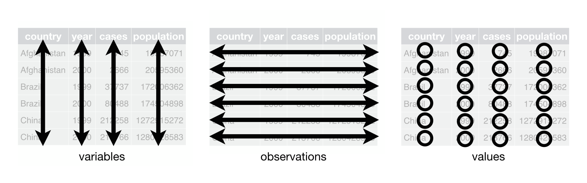R for Data Science, Wickham H and Grolemund G (https://r4ds.had.co.nz/index.html) © Wickham, Grolemund 2017 This image is licenced under Attribution-NonCommercial-NoDerivs 3.0 United States (CC-BY-NC-ND 3.0 US)

У цьому розділі ми розглянемо, як ці правила пов’язані з різними форматами даних, які зазвичай цікавлять дослідників: “широким” і “довгим”. Цей матеріал допоможе вам ефективно змінювати форму ваших даних незалежно від їх початкового формату. Спершу ми розглянемо характеристики даних interviews і те, як вони пов’язані з різними типами форматів даних.

Довгі та широкі формати даних

У наборі даних interviews кожен рядок містить значення змінних, пов’язаних із кожним записом (кожним інтерв’ю у селах). Зазначено, що key_ID “додано для надання унікального ідентифікатора для кожного спостереження”, а instanceID “робить те саме, але його не так зручно використовувати”.

Після того, як ми визначили, що key_ID і instanceID обидва є унікальними, ми можемо використовувати будь-яку з цих змінних як ідентифікатор для 131 запису інтерв’ю.

R

interviews %>% 
  select(key_ID) %>% 
  distinct() %>%
  nrow()

OUTPUT

[1] 131

Як видно з наведеного нижче коду, для кожної дати інтерв’ю в кожному селі instanceIDs не повторюються. Таким чином, цей формат називається “довгим” форматом даних, де кожне спостереження займає лише один рядок у датафреймі.

R

interviews %>%
  filter(village == "Chirodzo") %>%
  select(key_ID, village, interview_date, instanceID) %>%
  sample_n(size = 10)

OUTPUT

# A tibble: 10 × 4
   key_ID village  interview_date      instanceID
    <dbl> <chr>    <dttm>              <chr>
 1     35 Chirodzo 2016-11-17 00:00:00 uuid:ff7496e7-984a-47d3-a8a1-13618b5683ce
 2     54 Chirodzo 2016-11-16 00:00:00 uuid:273ab27f-9be3-4f3b-83c9-d3e1592de919
 3     63 Chirodzo 2016-11-16 00:00:00 uuid:86ed4328-7688-462f-aac7-d6518414526a
 4     60 Chirodzo 2016-11-16 00:00:00 uuid:85465caf-23e4-4283-bb72-a0ef30e30176
 5     44 Chirodzo 2016-11-17 00:00:00 uuid:f9fadf44-d040-4fca-86c1-2835f79c4952
 6     64 Chirodzo 2016-11-16 00:00:00 uuid:28cfd718-bf62-4d90-8100-55fafbe45d06
 7     62 Chirodzo 2016-11-16 00:00:00 uuid:c6597ecc-cc2a-4c35-a6dc-e62c71b345d6
 8      9 Chirodzo 2016-11-16 00:00:00 uuid:846103d2-b1db-4055-b502-9cd510bb7b37
 9     55 Chirodzo 2016-11-16 00:00:00 uuid:883c0433-9891-4121-bc63-744f082c1fa0
10     58 Chirodzo 2016-11-16 00:00:00 uuid:a7a3451f-cd0d-4027-82d9-8dcd1234fcca

Можемо помітити, що структура або формат даних interviews відповідає правилам 1-3, де

• кожен стовпець є змінною
• кожен ряд є спостереженням
• кожне значення має свою окрему клітинку

Це називають “довгим” форматом даних. Але зауважте, що кожен стовпець представляє різну змінну. У “найдовшому” форматі даних було б лише три стовпці: один для змінної-ідентифікатора, один для спостережуваної змінної та один для спостережуваного значення цієї змінної. Такий формат даних досить незручний і складний для роботи, тому його рідко використовують на практиці.

Крім того, у “широкому” форматі даних спостерігаються зміни в правилі 1: тепер кожен стовпець більше не обов’язково представляє лише одну змінну. Натомість стовпці можуть зображати різні рівні/значення змінної. Наприклад, у деяких наборах даних дослідники могли обрати, щоб кожна дата опитування була окремим стовпцем.

Хоча ці формати можуть здаватися радикально різними, існують інструменти, які роблять перехід між ними значно простішим, ніж може здатися! Гіф нижче показує, як ці два формати пов’язані між собою і дає уявлення про те, як можна використовувати R для переходу від одного формату до іншого.

Розташування даних у довгому та широкому форматах головним чином впливає на зручність перегляду. Візуально вам може більше подобатися “широкий” формат, оскільки на екрані можна побачити більше даних. Проте всі функції R, які ми використовували досі, очікують, що дані будуть у “довгому” форматі. Це пояснюється тим, що довгий формат легше сприймається машиною і ближчий до формату баз даних.

Питання, які вимагають різних форматів даних

У даних інтерв’ю кожен рядок містить значення змінних, пов’язаних із кожним записом (одиницею), такі як село респондента, кількість членів домогосподарства або тип стіни їхнього будинку. Такий формат дозволяє порівнювати окремі опитування, але що робити, якщо ми хочемо розглянути відмінності між домогосподарствами, згрупованими за різними типами власності?

Щоб полегшити таке порівняння, потрібно створити нову таблицю, де кожен рядок (одиниця) складатиметься зі значень змінних, пов’язаних із власністю (тобто items_owned). Практично це означає, що значення елементів у items_owned (наприклад, велосипед, радіо, стіл тощо) стануть назвами стовпців, а клітинки міститимуть значення TRUE або FALSE, залежно від того, чи має домогосподарство цей предмет.

Після створення такої таблиці ми можемо досліджувати взаємозв’язки всередині та між селами. Ключовий момент тут у тому, що ми все ще дотримуємося структури охайних даних, але переформатували дані відповідно до потрібних спостережень.

Крім того, якщо дати інтерв’ю розташовані у кількох стовпцях, а нас цікавить візуалізація того, як змінювалися конфлікти щодо зрошення з часом у кожному селі. Для цього потрібно, щоб дати інтерв’ю були включені в один стовпець, а не розкидані по кількох. Таким чином, нам потрібно перетворити назви стовпців на значення змінної.

Обидві ці трансформації можна виконати за допомогою двох функцій пакета tidyr: pivot_wider() та pivot_longer().

Перетворення у широкий формат

---

pivot_wider() має три основні аргументи:

1. дані
2. змінна names_from, значення якої стануть новими назвами стовпців.
3. змінна values_from, значення якої заповнюватимуть нові стовпці.

Додаткові аргументи включають values_fill, який, якщо його встановити, заповнює пропущені значення вказаним значенням.

Використаймо pivot_wider(), щоб перетворити interviews і створити нові стовпці для кожного предмета, яким володіє домогосподарство. У цій трансформації є кілька нових концепцій, тому розглянемо її крок за кроком. Спершу ми створимо новий об’єкт (interviews_items_owned) на основі датафрейму interviews.

R

interviews_items_owned <- interviews %>%

Тоді нам насправді потрібно зробити наш датафрейм довшим, тому що в одній клітинці міститься кілька предметів. Ми використаємо нову функцію separate_longer_delim() з пакета tidyr, щоб розділити значення змінної items_owned за наявністю крапок з комою (;). Значення цієї змінної містили кілька предметів, розділених крапками з комою, тому ця операція створює окремий рядок для кожного предмета, зазначеного у власності домогосподарства. Таким чином ми отримуємо довгу версію набору даних — з кількома рядками для кожного респондента. Наприклад, якщо респондент має телевізор і сонячну панель, то тепер у нього буде два рядки: один із “television”, а інший із “solar panel” у стовпці items_owned.

R

separate_longer_delim(items_owned, delim = ";") %>%

Після цього перетворення ви можете помітити, що в стовпці items_owned з’явилися значення NA. Це тому, що деякі респонденти не володіли жодним із предметів, зазначених у списку інтерв’юера. Ми можемо використати функцію replace_na(), щоб замінити ці NA на більш змістовне значення. Функція replace_na() очікує, що ви передасте їй list() зі стовпцями, у яких хочете замінити значення NA, а також значення, на яке потрібно замінити ці NA. У результаті це виглядає так:

R

replace_na(list(items_owned = "no_listed_items")) %>%

Далі ми створюємо нову змінну items_owned_logical, яка має значення (TRUE) для кожного рядка. Це логічно, адже кожен предмет у кожному рядку належав відповідному домогосподарству. Ми створюємо цю змінну для того, щоб під час розширення items_owned у кілька стовпців можна було заповнити їх логічними значеннями, які показують, чи володіло домогосподарство відповідним предметом (TRUE) або ні (FALSE).

R

mutate(items_owned_logical = TRUE) %>%

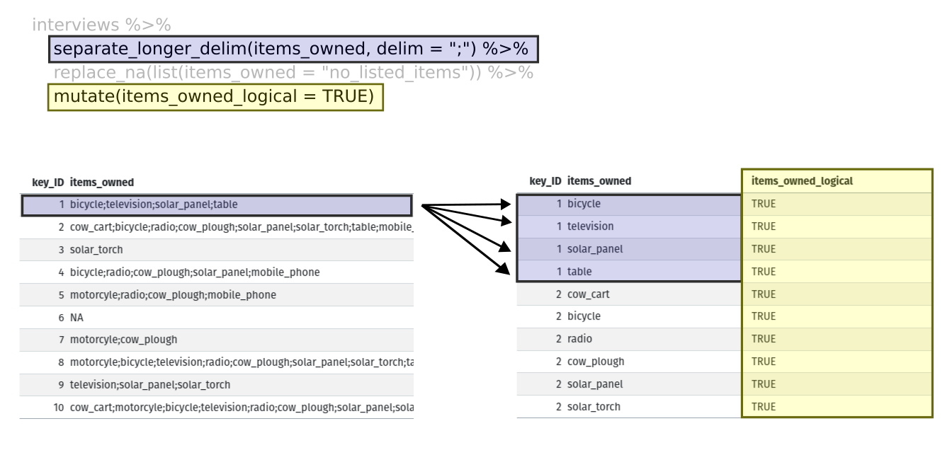
На цьому етапі ми також можемо порахувати кількість предметів, якими володіє кожне домогосподарство, що еквівалентно кількості рядків для кожного key_ID. Ми можемо зробити це за допомогою group_by() та mutate(), який працює схоже на комбінацію group_by() і summarize(), розглянуту в попередньому прикладі, але замість створення підсумкової таблиці ми додамо новий стовпець number_items. Для підрахунку кількості рядків у кожній групі використовується функція n(). Однак потрібно врахувати один момент: домогосподарства, які не зазначили жодного предмета. У цих домогосподарств тепер у стовпці items_owned зазначено "no_listed_items". Ми не хочемо рахувати це як предмет, тому замість цього потрібно поставити нуль. Цього можна досягти за допомогою функції if_else() з пакета dplyr, яка оцінює умову і повертає одне значення, якщо умова істинна, і інше — якщо хибна. Тут, якщо стовпець items_owned дорівнює "no_listed_items", повертається 0, інакше кількість рядків у групі повертається за допомогою n().

R

group_by(key_ID) %>% 
  mutate(number_items = if_else(items_owned == "no_listed_items", 0, n())) %>% 

Нарешті ми використовуємо pivot_wider(), щоб перейти з довгого формату в широкий. Це створює новий стовпець для кожного унікального значення у стовпці items_owned і заповнює ці стовпці значеннями з items_owned_logical. Крім того, ми вказуємо, що для відсутніх предметів клітинки потрібно заповнювати значенням FALSE замість NA.

R

pivot_wider(names_from = items_owned,
            values_from = items_owned_logical,
            values_fill = list(items_owned_logical = FALSE))

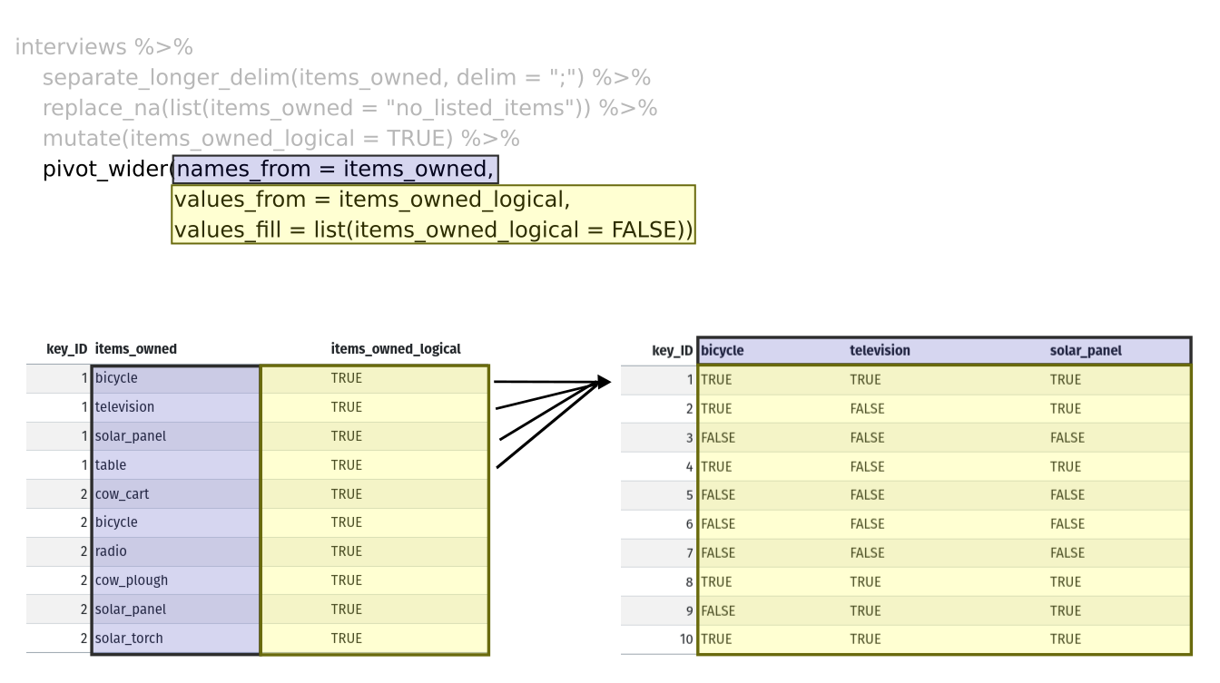
Об’єднавши наведені кроки, код виглядає так. Зверніть увагу, що два нові стовпці створюються в одному виклику mutate().

R

interviews_items_owned <- interviews %>%
  separate_longer_delim(items_owned, delim = ";") %>%
  replace_na(list(items_owned = "no_listed_items")) %>%
  group_by(key_ID) %>%
  mutate(items_owned_logical = TRUE,
         number_items = if_else(items_owned == "no_listed_items", 0, n())) %>%
  pivot_wider(names_from = items_owned,
              values_from = items_owned_logical,
              values_fill = list(items_owned_logical = FALSE))

Перегляньте дата фрейм interviews_items_owned. Він має rnrow(interviews) рядків (таку ж кількість, як і спочатку), але додаткові стовпці для кожного предмета. Скільки стовпців було додано? Зверніть увагу, що більше немає стовпця items_owned. Це тому, що в pivot_wider() за замовчуванням встановлено параметр, який видаляє оригінальний стовпець. Значення, які були в цьому стовпці, тепер стали стовпцями з назвами television, solar_panel, table тощо. Ви можете використати dim(interviews) та dim(interviews_wide), щоб побачити, як змінилася кількість стовпців між двома наборами даних.

Такий формат даних дозволяє виконувати цікаві операції, наприклад, створювати таблицю, що показує кількість респондентів у кожному селі, які володіли певним предметом:

R

interviews_items_owned %>%
  filter(bicycle) %>%
  group_by(village) %>%
  count(bicycle)

OUTPUT

# A tibble: 3 × 3
# Groups:   village [3]
  village  bicycle     n
  <chr>    <lgl>   <int>
1 Chirodzo TRUE       17
2 God      TRUE       23
3 Ruaca    TRUE       20

Або нижче ми обчислюємо середню кількість предметів зі списку, якими володіли респонденти в кожному селі, використовуючи стовпець number_items, який ми створили для підрахунку предметів у кожного домогосподарства.

R

interviews_items_owned %>%
    group_by(village) %>%
    summarize(mean_items = mean(number_items))

OUTPUT

# A tibble: 3 × 2
  village  mean_items
  <chr>         <dbl>
1 Chirodzo       4.54
2 God            3.98
3 Ruaca          5.57

Challenge

Завдання

Ми створили interviews_items_owned, переформатувавши дані: спочатку у довгий формат, а потім у широкий. Виконайте цей самий процес для стовпця months_lack_food у дата фрейміinterviews. Створіть новий дата фрейм зі стовпцями для кожного місяця, заповненими логічними значеннями (TRUEабоFALSE) та додайте підсумковий стовпецьnumber_months_lack_food`, який обчислює кількість місяців, протягом яких домогосподарство повідомляло про нестачу їжі.

Зверніть увагу: якщо домогосподарство не відчувало нестачі їжі протягом останніх 12 місяців, у стовпці було введено “none”.

Відповідь

R

months_lack_food <- interviews %>%
  separate_longer_delim(months_lack_food, delim = ";") %>%
  group_by(key_ID) %>%
  mutate(months_lack_food_logical = TRUE,
         number_months_lack_food = if_else(months_lack_food == "none", 0, n())) %>%
  pivot_wider(names_from = months_lack_food,
              values_from = months_lack_food_logical,
              values_fill = list(months_lack_food_logical = FALSE))

Перетворення у довгий формат

---

Протилежна ситуація може виникнути, якщо нам надали дані у форматі interviews_wide, де предмети, якими володіють домогосподарства, записані як назви стовпців, але ми хочемо розглядати їх як значення змінної items_owned.

У такій ситуації ми «збираємо» ці стовпці, перетворюючи їх на пару нових змінних. Одна змінна міститиме назви стовпців як значення, а інша — значення кожної клітинки, які раніше були пов’язані з цими назвами стовпців. Ми зробимо це у два кроки, щоб процес був зрозумілішим.

pivot_longer() приймає чотири основні аргументи:

1. дані
2. cols - назви стовпців, які ми використовуємо для заповнення нової змінної значень (або для видалення).
3. names_to - назва нової змінної, яку ми хочемо створити з наданих cols.
4. values_to — назва нової змінної, яку ми хочемо створити та заповнити значеннями, пов’язаними з наданими cols.

R

interviews_long <- interviews_items_owned %>%
  pivot_longer(cols = bicycle:car,
               names_to = "items_owned",
               values_to = "items_owned_logical")

Перегляньте обидва датафрейми interviews_long та interviews_items_owned і порівняйте їхню структуру.

Challenge

Завдання

Ми створили деякі підсумкові таблиці для interviews_items_owned за допомогою count та summarise. Ми можемо створити ті самі таблиці на основі interviews_long, але процес буде іншим.

Створіть таблицю, яка показує кількість респондентів у кожному селі, які володіли певним предметом, включаючи всі предмети. Різниця між цим форматом і широким форматом у тому, що тепер можна рахувати всі предмети, використовуючи змінну items_owned.

Відповідь

R

interviews_long %>%
  filter(items_owned_logical) %>% 
  group_by(village) %>% 
  count(items_owned)

OUTPUT

# A tibble: 47 × 3
# Groups:   village [3]
   village  items_owned         n
   <chr>    <chr>           <int>
 1 Chirodzo bicycle            17
 2 Chirodzo computer            2
 3 Chirodzo cow_cart            6
 4 Chirodzo cow_plough         20
 5 Chirodzo electricity         1
 6 Chirodzo fridge              1
 7 Chirodzo lorry               1
 8 Chirodzo mobile_phone       25
 9 Chirodzo motorcyle          13
10 Chirodzo no_listed_items     3
# ℹ 37 more rows

Застосування отриманих знань для очищення даних

---

Тепер ми одночасно ознайомилися з pivot_longer() та pivot_wider() і виправили проблему в структурі наших даних. У цьому наборі даних є ще один стовпець, який містить кілька значень в одній клітинці. Деякі клітинки стовпця months_lack_food містять кілька місяців, які, як і раніше, розділені крапкою з комою (;).

Щоб створити датафрейм, де кожен стовпець містить лише одне значення в клітинці, ми можемо повторити ті ж кроки, що застосовували для items_owned, і застосувати їх до months_lack_food. Оскільки цей датафрейм ми будемо використовувати в наступному розділі, назвемо його interviews_plotting.

R

## Візуалізація даних ##
interviews_plotting <- interviews %>%
  ## pivot wider by items_owned
  separate_longer_delim(items_owned, delim = ";") %>%
  replace_na(list(items_owned = "no_listed_items")) %>%
  ## Use of grouped mutate to find number of rows
  group_by(key_ID) %>% 
  mutate(items_owned_logical = TRUE,
         number_items = if_else(items_owned == "no_listed_items", 0, n())) %>% 
  pivot_wider(names_from = items_owned,
              values_from = items_owned_logical,
              values_fill = list(items_owned_logical = FALSE)) %>% 
  ## pivot wider by months_lack_food
  separate_longer_delim(months_lack_food, delim = ";") %>%
  mutate(months_lack_food_logical = TRUE,
         number_months_lack_food = if_else(months_lack_food == "none", 0, n())) %>%
  pivot_wider(names_from = months_lack_food,
              values_from = months_lack_food_logical,
              values_fill = list(months_lack_food_logical = FALSE))

Експорт даних

---

Тепер, коли ви навчилися використовувати dplyr та tidyr для обробки сирих даних, можливо, ви захочете експортувати ці нові набори даних, щоб поділитися ними з колегами або зберегти для архіву.

Подібно до функції read_csv(), яка використовується для зчитування CSV-файлів у R, існує функція write_csv(), яка дозволяє створювати CSV-файли з датафреймів.

Перед використанням write_csv() ми створимо нову теку data_output у нашій робочій директорії, куди будемо зберігати згенерований набір даних. Не слід записувати згенеровані набори даних у ту саму директорію, де зберігаються сирі дані. Хорошою практикою є тримати їх окремо. Тека data повинна містити лише сирі, незмінені дані, щоб уникнути їх випадкового видалення або зміни. Натомість скрипт буде створювати вміст теки data_output, тому навіть якщо файли там будуть видалені, їх завжди можна повторно згенерувати.

Для підготовки до наступного уроку з візуалізації ми створили версію набору даних, де кожен стовпець містить лише одне значення. Тепер ми можемо зберегти цей датафрейм у теку data_output.

R

write_csv(interviews_plotting, file = "data_output/interviews_plotting.csv")

Key Points

• Використовуйте пакет tidyr, щоб змінювати структуру датафреймів.
• Використовуйте pivot_width() для переходу від довгого до широкого формату.
• Використовуйте pivot_longer() для переходу від широкого до довгого формату.

Content from Візуалізація даних за допомогою ggplot2

---

Last updated on 2026-01-17 | Edit this page

Estimated time: 115 minutes

Instructor Note

• Цей епізод є загальним оглядом ggplot2 і зосереджується на: (1) ознайомленні з системою шарів у ggplot2, (2) використанні аргументу group у функції aes(), (3) базовому налаштуванні графіків.
• Епізод залежить від даних, створених в епізоді “Маніпулювання даними за допомогою tidyr”. Якщо ви не дійшли або не пройшли увесь епізод про tidyr, ви можете надати учасникам доступ до даних, завантаживши їх або швидко створивши за допомогою наведеного нижче коду tidyr. Ймовірно, ви захочете скопіювати код в Etherpad.
• Якщо ви пропустили епізод про tidyr, ви можете перейти до розділу експорт даних у тому епізоді.

Overview

Questions

• Які компоненти ggplot?
• Які основні відмінності між базовими графіками R, lattice та ggplot?
• Як створити діаграми розсіювання, коробкові та стовпчикові?
• Як змінити естетику (наприклад, колір, прозорість) графіка?
• Як створити кілька графіків одночасно?

Objectives

• Створити точкові, коробкові та стовпчикові діаграми за допомогою ggplot.
• Задати універсальні параметри графіка.
• Пояснити, що таке фасетування та застосувати його в ggplot.
• Змінити естетику наявного графіка ggplot (включно з підписами осей та кольором).
• Побудувати складні та персоналізовані графіки на основі даних у датафреймі.
• Визначити відмінності між візуалізаціями базового R, lattice та ggplot.

Почнемо із завантаження необхідного пакета. ggplot2 також входить до складу пакету tidyverse.

R

library(tidyverse)

Якщо дані ще не знаходяться в робочій області, завантажте ті, які ми зберегли в попередньому уроці.

R

interviews_plotting <- read_csv("data_output/interviews_plotting.csv")

OUTPUT

Rows: 131 Columns: 45
── Column specification ────────────────────────────────────────────────────────
Delimiter: ","
chr   (5): village, respondent_wall_type, memb_assoc, affect_conflicts, inst...
dbl   (8): key_ID, no_membrs, years_liv, rooms, liv_count, no_meals, number_...
lgl  (31): bicycle, television, solar_panel, table, cow_cart, radio, cow_plo...
dttm  (1): interview_date

ℹ Use `spec()` to retrieve the full column specification for this data.
ℹ Specify the column types or set `show_col_types = FALSE` to quiet this message.

Якщо ви не змогли завершити попередній урок або не зберегли дані, ви можете створити їх зараз. Або завантажте за допомогою read_csv() (варіант 1), або створіть за допомогою dplyr та tidyr (варіант 2).

Варіант 1: Завантажте дані

Варіант 2: Створіть дані

R

interviews_plotting <- read_csv("https://raw.githubusercontent.com/datacarpentry/r-socialsci/main/episodes/data/interviews_plotting.csv")

R

## Може бути використано для завантаження даних з попереднього уроку!
interviews_plotting <- interviews %>%
  ## pivot wider by items_owned
  separate_longer_delim(items_owned, delim = ";") %>%
  replace_na(list(items_owned = "no_listed_items")) %>%
  ## Use of grouped mutate to find number of rows
  group_by(key_ID) %>% 
  mutate(items_owned_logical = TRUE,
         number_items = if_else(items_owned == "no_listed_items", 0, n())) %>% 
  pivot_wider(names_from = items_owned,
              values_from = items_owned_logical,
              values_fill = list(items_owned_logical = FALSE)) %>% 
  ## pivot wider by months_lack_food
  separate_longer_delim(months_lack_food, delim = ";") %>%
  mutate(months_lack_food_logical = TRUE,
         number_months_lack_food = if_else(months_lack_food == "none", 0, n())) %>%
  pivot_wider(names_from = months_lack_food,
              values_from = months_lack_food_logical,
              values_fill = list(months_lack_food_logical = FALSE))

Параметри візуалізації в R

---

Перед тим як почати з ggplot2, корисно знати, що в R існує кілька способів створювати візуалізації. Хоча ggplot2 чудово підходить для створення складних та висококастомізованих графіків, існують простіші та швидші альтернативи, з якими ви можете зіткнутися або використовувати залежно від контексту. Давайте коротко розглянемо декілька з них:

Базові графіки R

Базові графіки R є найпростішою формою візуалізації й чудово підходять для швидкого, дослідницького аналізу. Можна створювати графіки за допомогою невеликої кількості коду, але їхнє налаштування може бути громіздким у порівнянні з ggplot2.

Приклад простого точкового графіка у базовому R з використанням змінних no_membrs та liv_count:

R

plot(interviews_plotting$no_membrs, interviews_plotting$liv_count,
     main = "Base R Scatterplot",
     xlab = "Number of Household Members",
     ylab = "Number of Livestock Owned")

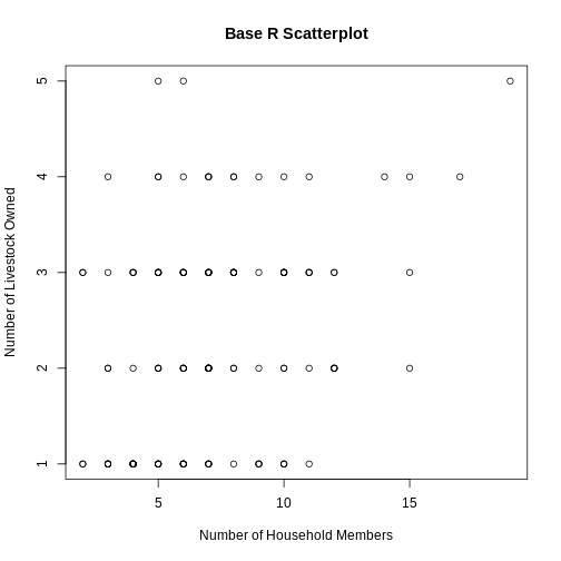
Lattice

Lattice — це ще одна система побудови графіків в R, яка дозволяє легко створювати багато панельні графіки у вигляді решітки. Воно відрізняється від ggplot2 тим, що весь графік визначається одним викликом функції та можливості для змін після побудови графіка обмежені.

Приклад графіка lattice з використанням змінних no_membrs та liv_count, розбитих за village:

R

library(lattice)

R

xyplot(liv_count ~ no_membrs | village, data = interviews_plotting,
       main = "Lattice Plot: Livestock Count by Household Members",
       xlab = "Number of Household Members",
       ylab = "Number of Livestock Owned")

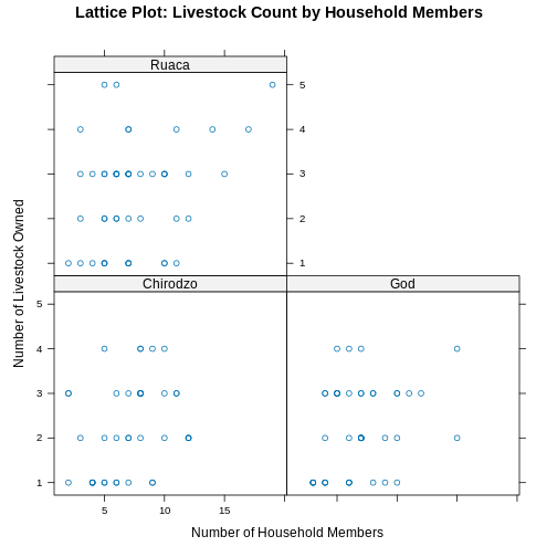
Побудова графіків за допомогою ggplot2

---

ggplot2 — це пакет для побудови графіків у R, який дозволяє легко створювати складні візуалізації з даних датафрейму. Він забезпечує програмний інтерфейс, який дозволяє задавати, які змінні зображати, як їх показувати та загальні візуальні властивості. Тому нам потрібно внести лише мінімальні зміни, якщо вихідні дані зміняться або якщо ми вирішимо перейти, наприклад, від стовпчикової діаграми до точкової (діаграма розсіювання). Це допомагає створювати графіки публікаційної якості з мінімальною кількістю коригувань і налаштувань.

Функції ggplot2 найкраще працюють із даними у ‘long’ форматі, тобто коли кожен вимір представлений окремим стовпцем, а кожне спостереження — окремим рядком. Добре структуровані дані заощадять вам багато часу під час побудови графіків у ggplot2

ggplot графіки будуються крок за кроком шляхом додавання нових елементів. Такий спосіб додавання шарів забезпечує велику гнучкість і дозволяє налаштовувати побудовані графіки.

Кожен графік, побудований за допомогою ggplot2, повинен включати такі елементи

• Дані

• Естетичне відображення (aes)

  • Описує як змінні накладаються на графічні атрибути
  • До таких атрибутів належать осі x і y, колір, заливка, форма точок, прозорість (alpha)

• Геометричні об’єкти (geom)

  • Визначає, як дані будуть зображені графічно — у вигляді стовпчиків (geom_bar), діаграми розсіювання (geom_point), лінії (geom_line) тощо.

Таким чином, шаблон побудови графіка в ggplot2:

<DATA> %>%
    ggplot(aes(<MAPPINGS>)) +
    <GEOM_FUNCTION>()

Нагадаємо з попереднього уроку, що оператор %>% (pipe) передає результат попереднього кроку як вхідні дані для наступної функції. ggplot — це функція, яка очікує датафрейм як перший аргумент. Це дозволяє не вказувати аргумент data = всередині функції ggplot, а просто передавати дані через pipe (%>%).

• використайте функцію ggplot() та прив’яжіть графік до певного датафрейму.

R

interviews_plotting %>%
    ggplot()

• визначити відображення (mapping) за допомогою функції aes(), обравши змінні для побудови графіка та вказавши, як їх показувати на графіку, наприклад, через позиції по осях x/y або через характеристики, такі як розмір, форма, колір тощо.

R

interviews_plotting %>%
    ggplot(aes(x = no_membrs, y = number_items))

• додати ‘geoms’ — графічні представлення даних на графіку (точки, лінії, стовпчики). ggplot2 пропонує багато різних geoms; сьогодні ми використаємо деякі з поширених, зокрема:

  • geom_point() для діаграм розсіювання, точкових графіків тощо.
  • geom_boxplot() для коробкових діаграм (boxplots)!
  • geom_line() для ліній тренду, часових рядів тощо.

Щоб додати geom до графіка, використовуйте оператор +. Оскільки у нас дві безперервні змінні, спочатку використаємо geom_point():

R

interviews_plotting %>%
    ggplot(aes(x = no_membrs, y = number_items)) +
    geom_point()

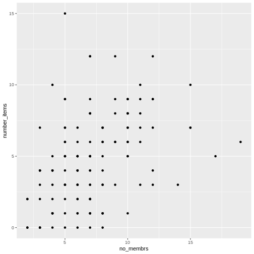
Символ + у пакеті ggplot2 особливо корисний, тому що він дозволяє змінювати вже створені об’єкти ggplot. Це означає, що ви можете легко налаштовувати шаблони графіків і зручно досліджувати різні типи візуалізацій, тому наведений вище графік також можна створити за допомогою такого коду, подібного до підходу “проміжних кроків” у попередньому уроці:

R

# Присвоїти графік змінній
interviews_plot <- interviews_plotting %>%
    ggplot(aes(x = no_membrs, y = number_items))

# Побудувати точковий графік
interviews_plot +
    geom_point()

Callout

Примітки

• Усе, що ви вказуєте у функції ggplot(), буде доступним для будь-яких шарів geom, які ви додаєте (тобто це універсальні налаштування графіка). Це включає відображення осей x та y, яке ви задали в aes().
• Ви також можете задавати відображення (mappings) окремо для конкретного geom, незалежно від того, що визначено глобально у функції ggplot().
• Знак +, який використовується для додавання нових шарів, має бути розміщений наприкінці рядка, що містить попередній шар. Якщо ж знак + поставити на початку рядка, де додається новий шар, то ggplot2 не додасть цей новий шар і поверне повідомлення про помилку.

R

## Це правильний синтаксис для додавання шарів
interviews_plot +
    geom_point()

## Це не додасть новий шар і поверне повідомлення про помилку
interviews_plot
+ geom_point()

Побудова графіків крок за кроком

---

Побудова графіків у ggplot2 зазвичай відбувається ітеративно. Спочатку ми визначаємо набір даних, який будемо використовувати, розмічаємо осі та обираємо geom:

R

interviews_plotting %>%
    ggplot(aes(x = no_membrs, y = number_items)) +
    geom_point()

Потім ми починаємо модифікувати цей графік, щоб витягти з нього більше інформації. Наприклад, при перегляді графіка ми помічаємо, що точки з’являються лише на перетині цілих чисел змінних no_membrs та number_items. Також, за приблизною оцінкою, здається, що на графіку значно менше точок, ніж рядків у нашому датафреймі. Це повинно нас привести до думки, що може бути кілька спостережень, накладених одне на одне (наприклад, три спостереження, де no_membrs = 3 і number_items = 1).

Існує два основні способи розв’язання проблеми накладення точок (overplotting):

1. зміна прозорості точок
2. злегка зсунути розташування точок

Спочатку розглянемо варіант 1 — зміну прозорості точок. Під “прозорістю” ми маємо на увазі непрозорість точки, тобто вашу здатність бачити крізь точку. Ми можемо керувати прозорістю точок за допомогою аргументу alpha у geom_point. Значення alpha варіюються від 0 до 1, причому менші значення роблять колір більш прозорим (alpha = 1 — значення за замовчуванням). Зокрема, alpha = 0.1 робить точку у десять разів прозорішою, ніж звичайна точка. Інакше кажучи, десять точок, накладених одна на одну, виглядатимуть як звичайна точка.

Тут ми змінюємо alpha на alpha, намагаючись зменшити ефект накладення точок. Хоча проблему накладення точок повністю не вирішено, додавання прозорості починає її зменшувати, оскільки точки, де спостереження накладаються, виглядають темнішими (на відміну від світло-сірих):

R

interviews_plotting %>%
    ggplot(aes(x = no_membrs, y = number_items)) +
    geom_point(alpha = 0.5)

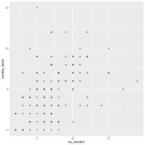
Це лише трохи допомогло з проблемою накладення точок, тому спробуємо другий варіант. Ми можемо злегка змістити точки на графіку, щоб бачити кожну точку навіть у місцях, де вони накладаються. Це зміщення додає трохи випадковості у розташування наших точок. Можна уявити цей процес як легке струшування графіка з накладеними точками. Точки трохи зсуватимуться вліво-вправо та вгору-вниз, але їхнє положення на графіку значно не зміниться. Зверніть увагу, що цей спосіб підходить для цілих чисел, а для чисел з десятковими знаками geom_jitter() не підходить, оскільки спотворює справжнє значення спостереження.

Ми можемо зсунути точки за допомогою функції geom_jitter() замість geom_point(), як показано нижче:

R

interviews_plotting %>%
    ggplot(aes(x = no_membrs, y = number_items)) +
    geom_jitter()

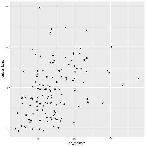
Функція geom_jitter() дозволяє задати величину випадкового зсуву за допомогою аргументів width і height. Якщо не вказувати значення для width і height, geom_jitter() за замовчуванням використовує 40% від роздільної здатності даних (найменша зміна, яку можна виміряти). Тому, якщо ми хочемо менший зсув (jitter), ніж за замовчуванням, слід обрати значення між 0.1 та 0.4. Експериментуйте зі значеннями, щоб побачити, як змінюється ваш графік.

R

interviews_plotting %>%
    ggplot(aes(x = no_membrs, y = number_items)) +
    geom_jitter(alpha = 0.5,
                width = 0.2,
                height = 0.2)

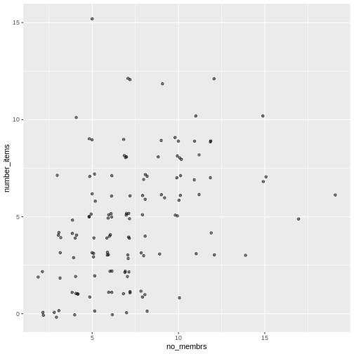
Для останньої зміни ми можемо також додати кольори всім точкам, вказавши аргумент color всередині функції geom_jitter():

R

interviews_plotting %>%
    ggplot(aes(x = no_membrs, y = number_items)) +
    geom_jitter(alpha = 0.5,
                color = "blue",
                width = 0.2,
                height = 0.2)

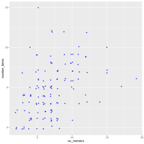
Щоб по-різному зафарбувати кожне село на графіку, можна передати в аргумент color вектор. Однак, оскільки ми тепер відображаємо ознаки даних через колір, замість того, щоб встановлювати один колір для всіх точок, колір точок слід вказувати всередині функції aes. Коли ми відображаємо змінну через колір точок, ggplot2 автоматично надає різні кольори для різних значень цієї змінної. Ми продовжимо задання значень alpha, width та height поза функцією aes, оскільки використовуємо одне й те саме значення для всіх точок. ggplot2 розуміє як британське, так і американське написання слова колір, тобто можна використовувати або color, або colour. Ось приклад, де ми фарбуємо точки залежно від village (села) спостереження:

R

interviews_plotting %>%
    ggplot(aes(x = no_membrs, y = number_items)) +
    geom_jitter(aes(color = village), alpha = 0.5, width = 0.2, height = 0.2)

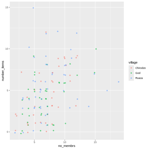
Схоже, що існує позитивна залежність між кількістю членів домогосподарства та кількістю придбаних предметів (з наведеного списку). Крім того, ця залежність, здається, не відрізняється між селами.

Callout

Примітки

Як ви дізнаєтеся, існує кілька способів зобразити залежність між змінними. Ще один спосіб побудови графіка з накладенням точок — використовувати функцію geom_count. Функція geom_count() робить розмір кожної точки пропорційним кількості елементів даних цього типу, а легенда показує, які розміри точок відповідають певній кількості елементів.

R

interviews_plotting %>%
   ggplot(aes(x = no_membrs, y = number_items, color = village)) +
   geom_count()

Challenge

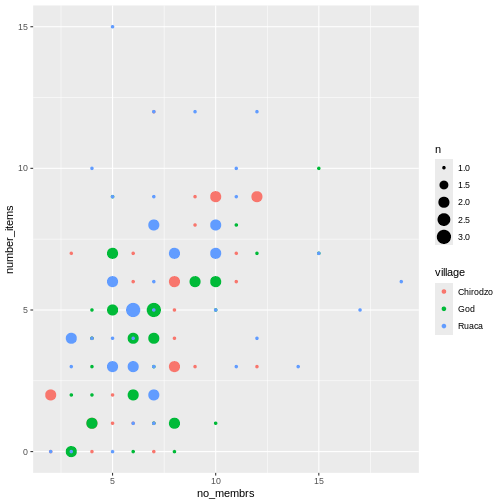
Завдання

Використайте щойно вивчене, щоб створити діаграму розсіювання (scatter plot) для rooms за village, де respondent_wall_type буде зображатися різними кольорами. Чи здається вам, що це гарний спосіб показати залежність між цими змінними? Які ще типи графіків можна використати для зображення такого типу даних?

Відповідь

R

interviews_plotting %>%
    ggplot(aes(x = village, y = rooms)) +
    geom_jitter(aes(color = respondent_wall_type),
      alpha = 0.5,
        width = 0.2,
        height = 0.2)

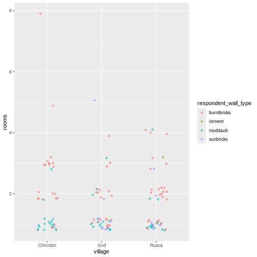
Це не дуже зручний спосіб показати такі дані, оскільки важко розрізнити села. Які ще типи графіків могли б краще допомогти вам візуалізувати цю залежність?

Коробковий графік (boxplot)

---

Ми можемо використовувати коробкові графіки (boxplots), щоб візуалізувати розподіл кімнат для кожного типу стін:

R

interviews_plotting %>%
    ggplot(aes(x = respondent_wall_type, y = rooms)) +
    geom_boxplot()

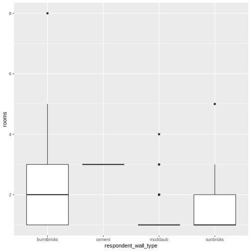
Додавши точки на boxplot, ми можемо краще уявити кількість вимірювань та їх розподіл:

R

interviews_plotting %>%
    ggplot(aes(x = respondent_wall_type, y = rooms)) +
    geom_boxplot(alpha = 0) +
    geom_jitter(alpha = 0.5,
        color = "tomato",
        width = 0.2,
        height = 0.2)

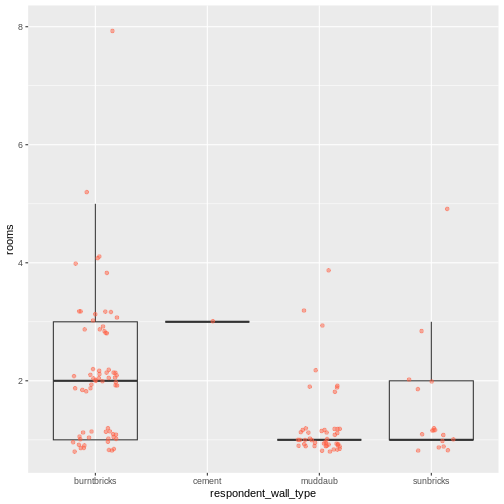
Ми бачимо, що будинки з глини (muddaub) та сонячної цегли (sunbrick) зазвичай менші за будинки з обпаленої цегли (burntbrick).

Зверніть увагу, як шар boxplot знаходиться позаду шару jitter? Що потрібно змінити в коді, щоб шар boxplot був попереду шару jitter?

Challenge

Завдання

Boxplot корисні для підсумкової інформації, але вони приховують форму розподілу. Наприклад, якщо розподіл бімодальний, ми цього не побачимо у boxplot. Альтернатива boxplot — це violin plot (скрипковий графік), де зображається форма розподілу точок (щільність даних).

• Замініть коробковий графік (boxplot) на скрипковий (violin plot); використайте geom_violin().

Відповідь

R

interviews_plotting %>%
  ggplot(aes(x = respondent_wall_type, y = rooms)) +
  geom_violin(alpha = 0) +
  geom_jitter(alpha = 0.5, color = "tomato")

WARNING

Warning: Groups with fewer than two datapoints have been dropped.
ℹ Set `drop = FALSE` to consider such groups for position adjustment purposes.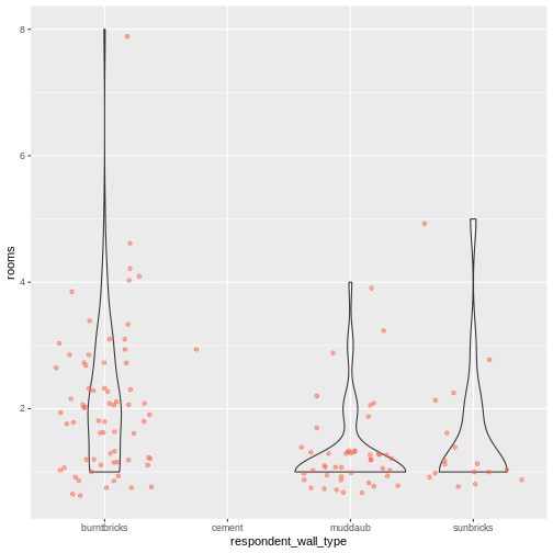

Challenge

Завдання (continued)

До цього моменту ми розглядали розподіл кількості кімнат у залежності від типу стін. Спробуйте створити новий графік, щоб дослідити розподіл іншої змінної залежно від типу стін.

• Створіть boxplot для liv_count для кожного типу стін. Накладіть шар boxplot на шар jitter, щоб показати фактичні вимірювання.

Відповідь

R

interviews_plotting %>%
   ggplot(aes(x = respondent_wall_type, y = liv_count)) +
   geom_boxplot(alpha = 0) +
   geom_jitter(alpha = 0.5, width = 0.2, height = 0.2)

Challenge

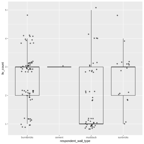
Завдання (continued)

• Додайте колір до точок на boxplot залежно від того, чи є респондент членом іригаційної асоціації (memb_assoc).

Відповідь

R

interviews_plotting %>%
  ggplot(aes(x = respondent_wall_type, y = liv_count)) +
  geom_boxplot(alpha = 0) +
  geom_jitter(aes(color = memb_assoc), alpha = 0.5, width = 0.2, height = 0.2)

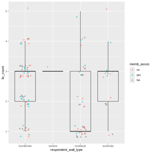
Стовпчасті діаграми (barplots)

---

Стовпчасті діаграми (barplots) також корисні для візуалізації категоріальних даних. За замовчуванням geom_bar приймає змінну для осі x і показує кількість випадків, з якими кожне значення x (у цьому випадку — тип стін) зустрічається в наборі даних.

R

interviews_plotting %>%
    ggplot(aes(x = respondent_wall_type)) +
    geom_bar()

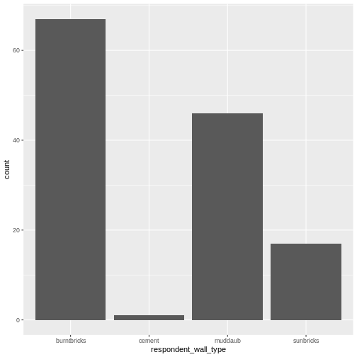
Ми можемо використати естетику fill у geom_bar(), щоб зафарбувати стовпчики відповідно до частки кожного підрахунку з кожного села.

R

interviews_plotting %>%
    ggplot(aes(x = respondent_wall_type)) +
    geom_bar(aes(fill = village))

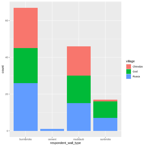
Це створює стовпчасту діаграму. Як правило, їх складніше читати, ніж стовпчики розташовані поруч. Ми можемо розділити частини складеної стовпчастої діаграми, що відповідають кожному селу і розмістити їх поруч, використавши аргумент position у geom_bar() та встановивши його значення “dodge”.

R

interviews_plotting %>%
    ggplot(aes(x = respondent_wall_type)) +
    geom_bar(aes(fill = village), position = "dodge")

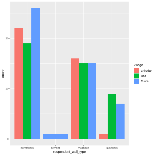
Це більш наочний графік, але нас, ймовірно, більше цікавить частка кожного типу житла в кожному селі, ніж фактична кількість будинків кожного типу (оскільки в різних селах могла бути опитана різна кількість домогосподарств). Щоб порівняти частки, ми спочатку створимо новий датафрейм (percent_wall_type) з новим стовпцем “percent”, який представляє відсоток кожного типу будинку в кожному селі. Також ми виключимо будинки з цементними стінами, оскільки в наборі даних був лише один такий будинок.

R

percent_wall_type <- interviews_plotting %>%
    filter(respondent_wall_type != "cement") %>%
    count(village, respondent_wall_type) %>%
    group_by(village) %>%
    mutate(percent = (n / sum(n)) * 100) %>%
    ungroup()

Тепер ми можемо використати цей новий датафрейм, щоб побудувати графік, який показує відсоток кожного типу будинку в кожному селі.

R

percent_wall_type %>%
    ggplot(aes(x = village, y = percent, fill = respondent_wall_type)) +
    geom_bar(stat = "identity", position = "dodge")

Challenge

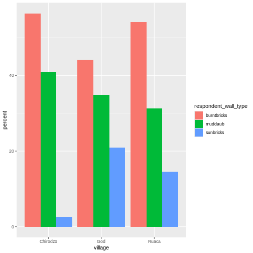
Завдання

Створіть стовпчасту діаграму, яка показує частку респондентів у кожному селі, які є або не є членами іригаційної асоціації (memb_assoc). У розрахунках і на графіку враховуйте лише тих респондентів, які відповіли на це запитання. Яке село має найменшу частку респондентів, що є членами іригаційної асоціації?

Відповідь

R

percent_memb_assoc <- interviews_plotting %>%
  filter(!is.na(memb_assoc)) %>%
  count(village, memb_assoc) %>%
  group_by(village) %>%
  mutate(percent = (n / sum(n)) * 100) %>%
  ungroup()

percent_memb_assoc %>%
   ggplot(aes(x = village, y = percent, fill = memb_assoc)) +
    geom_bar(stat = "identity", position = "dodge")

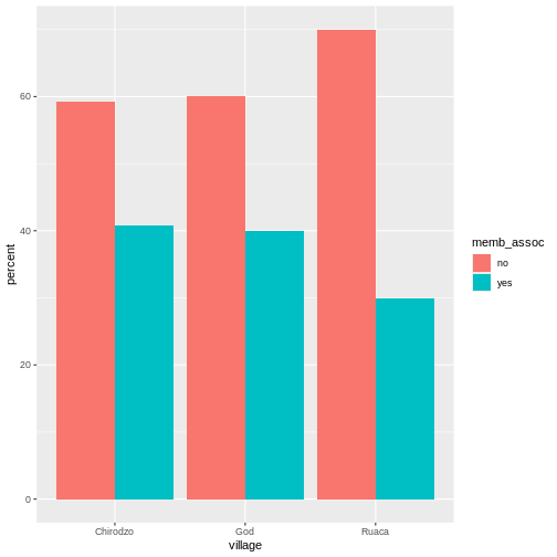
Село Ruaca мало найменшу частку респондентів, які є членами іригаційної асоціації.

Додавання підписів і заголовків

---

За замовчуванням підписи осей на графіку беруться з назв змінних, які ми зображаємо. Проте, ggplot2 пропонує багато можливостей для налаштування: можна задавати власні підписи осей, додавати заголовок до графіка за допомогою відносно невеликої кількості коду. Ми додамо більш інформативні підписи для осей x та y, пояснювальний підпис для легенди та заголовок до графіка.

Функція labs приймає такі аргументи:

• title – заголовок графіку
• subtitle – підзаголовок (текст меншим шрифтом під заголовком)
• caption – підпис до графіка
• ... – будь-які пари імені та значення для естетики, які використовуються у графіку (наприклад, x, y, fill, color, size)

R

percent_wall_type %>%
    ggplot(aes(x = village, y = percent, fill = respondent_wall_type)) +
    geom_bar(stat = "identity", position = "dodge") +
    labs(title = "Proportion of wall type by village",
         fill = "Type of Wall in Home",
         x = "Village",
         y = "Percent")

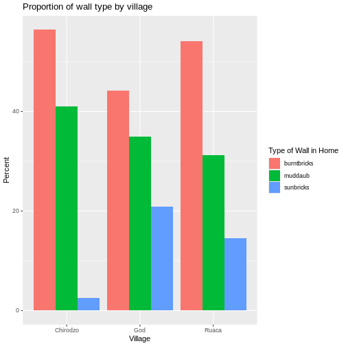
Фасетування

---

Замість того, щоб створювати один графік зі стовпчиками поруч для кожної громади, ми можемо створити кілька графіків, де кожен показує дані для однієї громади. Це особливо корисно, якщо у нас велика кількість громад у вибірці, адже багато стовпчиків поруч важко читати.

У ggplot2 є спеціальна техніка, яка називається faceting (фасетування), яка дозволяє розбити один графік на кілька графіків на основі факторної змінної у наборі даних. Ми використаємо її, щоб розбити наш стовпчастий графік пропорцій типів будинків за громадами так, щоб для кожної громади був власна панель у багатопанельному графіку:

R

percent_wall_type %>%
    ggplot(aes(x = respondent_wall_type, y = percent)) +
    geom_bar(stat = "identity", position = "dodge") +
    labs(title="Proportion of wall type by village",
         x="Wall Type",
         y="Percent") +
    facet_wrap(~ village)

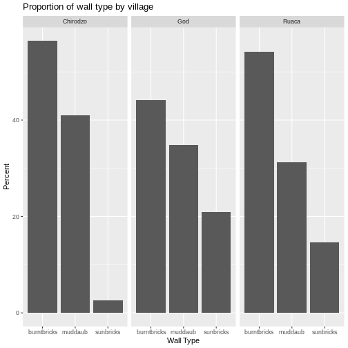
Натисніть кнопку “Zoom” у панелі графіків RStudio, щоб переглянути більшу версію цього графіка.

Зазвичай графіки на білому фоні легше читати при друку. Ми можемо встановити білий фон за допомогою функції theme_bw(). Крім того, можна прибрати сітку:

R

percent_wall_type %>%
    ggplot(aes(x = respondent_wall_type, y = percent)) +
    geom_bar(stat = "identity", position = "dodge") +
    labs(title="Proportion of wall type by village",
         x="Wall Type",
         y="Percent") +
    facet_wrap(~ village) +
    theme_bw() +
    theme(panel.grid = element_blank())

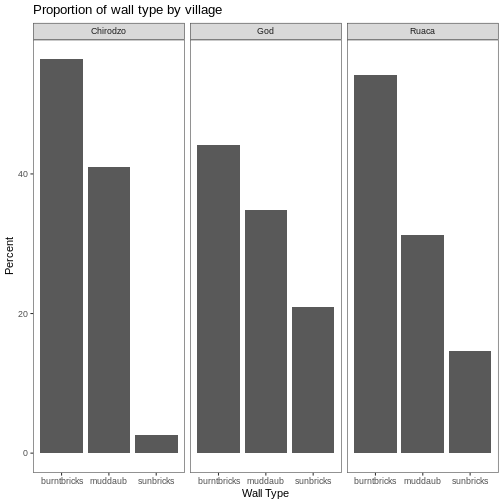
А що як ми хочемо побачити частку респондентів у кожному селі, які володіють певним предметом? Ми можемо порахувати відсоток людей у кожному селі, які мають кожен предмет, а потім створити серію фасетованих стовпчикових діаграм, де кожна діаграма відповідає окремому предмету. Спершу потрібно обчислити відсоток людей у кожному селі, які володіють кожним предметом:

R

percent_items <- interviews_plotting %>%
    group_by(village) %>%
    summarize(across(bicycle:no_listed_items, ~ sum(.x) / n() * 100)) %>%
    pivot_longer(bicycle:no_listed_items, names_to = "items", values_to = "percent")

Щоб обчислити цей датафрейм із відсотками, нам потрібно було використати функцію across() всередині операції summarize(). На відміну від попереднього прикладу з однією змінною типу стіни, де кожна відповідь належала лише до одного з типів, люди можуть (і часто мають) більше ніж один предмет. Тому у нас є кілька стовпців даних (по одному на кожен предмет) і обчислення відсотка потрібно повторити для кожної колонки.

Поєднання summarize() з across() дозволяє спочатку вказати стовпці, які потрібно підсумувати (bicycle:no_listed_items), а потім — обчислення. Оскільки наше обчислення трохи складніше, ніж доступні вбудовані функції, ми визначаємо нову формулу:

• ~ вказує, що ми визначаємо формулу,
• sum(.x) рахує кількість людей, які мають цей предмет, враховуючи значення TRUE(.x — це скорочення для стовпця, над яким виконується операція),
• і n() повертає розмір поточної групи.

Після операції summarize() ми отримуємо таблицю відсотків, де кожен предмет у власному стовпці, тому потрібне застосування pivot_longer(), щоб перетворити таблицю у зручніший формат для побудови графіка. Використовуючи цей датафрейм, ми можемо створити багатопанельну стовпчасту діаграму.

R

percent_items %>%
    ggplot(aes(x = village, y = percent)) +
    geom_bar(stat = "identity", position = "dodge") +
    facet_wrap(~ items) +
    theme_bw() +
    theme(panel.grid = element_blank())

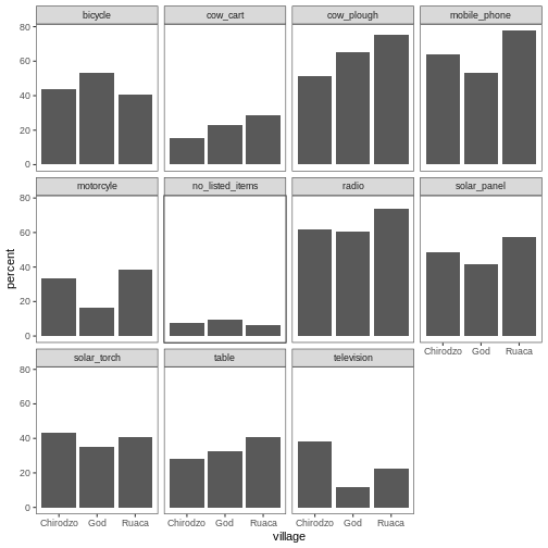
Теми в ggplot2

---

Окрім theme_bw(), яка змінює фон графіка на білий, ggplot2 має кілька інших тем, що дозволяють швидко змінювати вигляд візуалізації. Повний список тем доступний за посиланням: https://ggplot2.tidyverse.org/reference/ggtheme.html. theme_minimal() і theme_light() є популярними, а theme_void() може стати корисною відправною точкою для створення власної, ручної теми.

Пакет ggthemes пропонує великий вибір тем (включно з темою Excel 2003). Сайт розширень ggplot2 пропонує список пакетів, які розширюють можливості ggplot2, включно з додатковими темами.

Discussion

Завдання

Спробуйте використати щонайменше дві різні теми. Побудуйте попередній графік з кожною з цих тем. Яка вам подобається більше?

Налаштування

---

Подивіться на ggplot2 шпаргалку та подумайте, як можна покращити графік.

Тепер нумо змінимо назви осей на більш інформативні замість ‘village’ та ‘percent’ і додамо заголовок до графіка:

R

percent_items %>%
    ggplot(aes(x = village, y = percent)) +
    geom_bar(stat = "identity", position = "dodge") +
    facet_wrap(~ items) +
    labs(title = "Percent of respondents in each village who owned each item",
         x = "Village",
         y = "Percent of Respondents") +
    theme_bw()

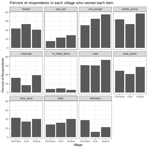
Назви осей стали більш інформативними, але їхню читабельність можна покращити, збільшивши розмір шрифту:

R

percent_items %>%
    ggplot(aes(x = village, y = percent)) +
    geom_bar(stat = "identity", position = "dodge") +
    facet_wrap(~ items) +
    labs(title = "Percent of respondents in each village who owned each item",
         x = "Village",
         y = "Percent of Respondents") +
    theme_bw() +
    theme(text = element_text(size = 16))

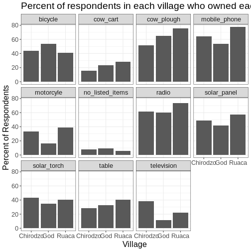
Зверніть увагу, що також можна змінювати шрифти на графіках. Якщо ви користуєтеся Windows, можливо, доведеться встановити пакет extrafont та дотримуватися інструкцій у README цього пакета.

Після наших змін можна помітити, що значення на осі x все ще не зовсім зручні для читання. Змінімо орієнтацію підписів і відрегулюємо їх вертикально та горизонтально, щоб вони не перекривалися. Можна використати кут 90 градусів або підібрати відповідний кут для діагонального розташування підписів. З більшим шрифтом заголовок теж може виходити за межі графіка. Ми можемо додати “\n” у рядок заголовка, щоб вставити новий рядок:

R

percent_items %>%
    ggplot(aes(x = village, y = percent)) +
    geom_bar(stat = "identity", position = "dodge") +
    facet_wrap(~ items) +
    labs(title = "Percent of respondents in each village \n who owned each item",
         x = "Village",
         y = "Percent of Respondents") +
    theme_bw() +
    theme(axis.text.x = element_text(colour = "grey20", size = 12, angle = 45,
                                     hjust = 0.5, vjust = 0.5),
          axis.text.y = element_text(colour = "grey20", size = 12),
          text = element_text(size = 16))

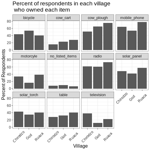
Якщо вам більше подобаються створені зміни у порівнянні з темою за замовчуванням, їх можна зберегти як об’єкт, щоб легко застосовувати до інших графіків, які ви створюватимете. Також можна додати plot.title = element_text(hjust = 0.5), щоб вирівняти заголовок по центру:

R

grey_theme <- theme(axis.text.x = element_text(colour = "grey20", size = 12,
                                               angle = 45, hjust = 0.5,
                                               vjust = 0.5),
                    axis.text.y = element_text(colour = "grey20", size = 12),
                    text = element_text(size = 16),
                    plot.title = element_text(hjust = 0.5))


percent_items %>%
    ggplot(aes(x = village, y = percent)) +
    geom_bar(stat = "identity", position = "dodge") +
    facet_wrap(~ items) +
    labs(title = "Percent of respondents in each village \n who owned each item",
         x = "Village",
         y = "Percent of Respondents") +
    grey_theme

Discussion

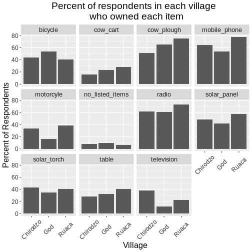
Завдання

Маючи всю цю інформацію, виділіть ще п’ять хвилин, щоб покращити один із графіків, створених у цьому завданні або створити власний гарний графік. Використайте RStudio шпаргалку ggplot2 для натхнення. Ось кілька ідей:

• Спробуйте зробити стовпці білими з чорним контуром.
• Спробуйте використати іншу кольорову палітру (див. http://www.cookbook-r.com/Graphs/Colors_(ggplot2)/).

Після створення графіка його можна зберегти у файл у потрібному форматі. Вкладка Export у вікні Plot в RStudio зберігає графіки у низькій роздільній здатності, що не підійде для більшості журналів і погано масштабується для постерів.

Замість цього використовуйте функцію ggsave(), яка дозволяє легко змінювати розмір і роздільну здатність графіка, налаштовуючи відповідні аргументи (width, height і dpi).

Переконайтеся, що у вашій робочій директорії є тека fig_output/.

R

my_plot <- percent_items %>%
    ggplot(aes(x = village, y = percent)) +
    geom_bar(stat = "identity", position = "dodge") +
    facet_wrap(~ items) +
    labs(title = "Percent of respondents in each village \n who owned each item",
         x = "Village",
         y = "Percent of Respondents") +
    theme_bw() +
    theme(axis.text.x = element_text(color = "grey20", size = 12, angle = 45,
                                     hjust = 0.5, vjust = 0.5),
          axis.text.y = element_text(color = "grey20", size = 12),
          text = element_text(size = 16),
          plot.title = element_text(hjust = 0.5))

ggsave("fig_output/name_of_file.png", my_plot, width = 15, height = 10)

Примітка: параметри width і hight також визначають розмір шрифту на збереженому графіку.

Key Points

• ggplot2 є гнучким та корисним інструментом для створення графіків у R.
• Набір даних і систему координат можна визначити за допомогою функції ggplot.
• Додаткові шари, включно з geoms, додаються за допомогою оператора +.
• Boxplot (коробковий графік) корисний для візуалізації розподілу числової змінної.
• Barplot (стовпчастий графік) зручний для візуалізації категоріальних даних.
• Faceting (фасетування) дозволяє створювати кілька графіків на основі категоріальної змінної.

Content from Getting started with R Markdown (Optional)

---

Last updated on 2025-12-15 | Edit this page

Estimated time: 45 minutes

Instructor Note

• This is an optional lesson intended to introduce learners to R Markdown.
• While it is listed after the core lessons, some instructors may prefer to teach it early in the workshop, depending on the audience.

Overview

Questions

• What is R Markdown?
• How can I integrate my R code with text and plots?
• How can I convert .Rmd files to .html?

Objectives

• Create a .Rmd document containing R code, text, and plots
• Create a YAML header to control output
• Understand basic syntax of (R)Markdown
• Customise code chunks to control formatting
• Use code chunks and in-line code to create dynamic, reproducible documents

R Markdown

---

R Markdown is a flexible type of document that allows you to seamlessly combine executable R code, and its output, with text in a single document. These documents can be readily converted to multiple static and dynamic output formats, including PDF (.pdf), Word (.docx), and HTML (.html).

The benefit of a well-prepared R Markdown document is full reproducibility. This also means that, if you notice a data transcription error, or you are able to add more data to your analysis, you will be able to recompile the report without making any changes in the actual document.

The rmarkdown package comes pre-installed with RStudio, so no action is necessary.

Image credit: Allison Horst

Creating an R Markdown file

---

To create a new R Markdown document in RStudio, click File -> New File -> R Markdown:

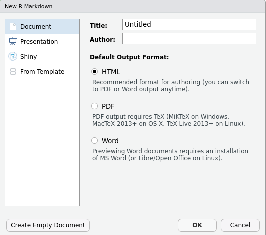
Then click on ‘Create Empty Document’. Normally you could enter the title of your document, your name (Author), and select the type of output, but we will be learning how to start from a blank document.

Basic components of R Markdown

---

To control the output, a YAML (YAML Ain’t Markup Language) header is needed:

---
title: "My Awesome Report"
author: "Emmet Brickowski"
date: ""
output: html_document
---

The header is defined by the three hyphens at the beginning (---) and the three hyphens at the end (---).

In the YAML, the only required field is the output:, which specifies the type of output you want. This can be an html_document, a pdf_document, or a word_document. We will start with an HTML doument and discuss the other options later.

The rest of the fields can be deleted, if you don’t need them. After the header, to begin the body of the document, you start typing after the end of the YAML header (i.e. after the second ---).

Markdown syntax

---

Markdown is a popular markup language that allows you to add formatting elements to text, such as bold, italics, and code. The formatting will not be immediately visible in a markdown (.md) document, like you would see in a Word document. Rather, you add Markdown syntax to the text, which can then be converted to various other files that can translate the Markdown syntax. Markdown is useful because it is lightweight, flexible, and platform independent.

Some platforms provide a real time preview of the formatting, like RStudio’s visual markdown editor (available from version 1.4).

First, let’s create a heading! A # in front of text indicates to Markdown that this text is a heading. Adding more #s make the heading smaller, i.e. one # is a first level heading, two ##s is a second level heading, etc. upto the 6th level heading.

# Title
## Section
### Sub-section
#### Sub-sub section
##### Sub-sub-sub section
###### Sub-sub-sub-sub section

(only use a level if the one above is also in use)

Since we have already defined our title in the YAML header, we will use a section heading to create an Introduction section.

## Introduction

You can make things bold by surrounding the word with double asterisks, **bold**, or double underscores, __bold__; and italicize using single asterisks, *italics*, or single underscores, _italics_.

You can also combine bold and italics to write something really important with triple-asterisks, ***really***, or underscores, ___really___; and, if you’re feeling bold (pun intended), you can also use a combination of asterisks and underscores, **_really_**, **_really_**.

To create code-type font, surround the word with backticks, `code-type`.

Now that we’ve learned a couple of things, it might be useful to implement them:

## Introduction

This report uses the **tidyverse** package along with the *SAFI* dataset,
which has columns that include:

Then we can create a list for the variables using -, +, or * keys.

## Introduction

This report uses the **tidyverse** package along with the *SAFI* dataset,
which has columns that include:

- village
- interview_date
- no_members
- years_liv
- respondent_wall_type
- rooms

You can also create an ordered list using numbers:

1. village
2. interview_date
3. no_members
4. years_liv
5. respondent_wall_type
6. rooms

And nested items by tab-indenting:

- village
  + Name of village
- interview_date
  + Date of interview
- no_members
  + How many family members lived in a house
- years_liv
  + How many years respondent has lived in village or neighbouring village
- respondent_wall_type
  + Type of wall of house
- rooms
  + Number of rooms in house

For more Markdown syntax see the following reference guide.

Now we can render the document into HTML by clicking the Knit button in the top of the Source pane (top left), or use the keyboard shortcut Ctrl+Shift+K on Windows and Linux, and Cmd+Shift+K on Mac. If you haven’t saved the document yet, you will be prompted to do so when you Knit for the first time.

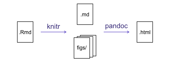
Writing an R Markdown report

---

Now we will add some R code from our previous data wrangling and visualisation, which means we need to make sure tidyverse is loaded. It is not enough to load tidyverse from the console, we will need to load it within our R Markdown document. The same applies to our data. To load these, we will need to create a ‘code chunk’ at the top of our document (below the YAML header).

A code chunk can be inserted by clicking Code > Insert Chunk, or by using the keyboard shortcuts Ctrl+Alt+I on Windows and Linux, and Cmd+Option+I on Mac.

The syntax of a code chunk is:

MARKDOWN

```{r chunk-name}
"Here is where you place the R code that you want to run."
```

An R Markdown document knows that this text is not part of the report from the ``` that begins and ends the chunk. It also knows that the code inside of the chunk is R code from the r inside of the curly braces ({}). After the r you can add a name for the code chunk . Naming a chunk is optional, but recommended. Each chunk name must be unique, and only contain alphanumeric characters and -.

To load tidyverse and our SAFI_clean.csv file, we will insert a chunk and call it ‘setup’. Since we don’t want this code or the output to show in our knitted HTML document, we add an include = FALSE option after the code chunk name ({r setup, include = FALSE}).

MARKDOWN

```{r setup, include = FALSE}
library(tidyverse)
library(here)
interviews <- read_csv(here("data/SAFI_clean.csv"), na = "NULL")
```

Callout

Important Note!

The file paths you give in a .Rmd document, e.g. to load a .csv file, are relative to the .Rmd document, not the project root.

As suggested in the Starting with Data episode, we highly recommend the use of the here() function to keep the file paths consistent within your project.

Insert table

---

Next, we will re-create a table from the Data Wrangling episode which shows the average household size grouped by village and memb_assoc. We can do this by creating a new code chunk and calling it ‘interview-tbl’. Or, you can come up with something more creative (just remember to stick to the naming rules).

It isn’t necessary to Knit your document every time you want to see the output. Instead you can run the code chunk with the green triangle in the top right corner of the the chunk, or with the keyboard shortcuts: Ctrl+Alt+C on Windows and Linux, or Cmd+Option+C on Mac.

To make sure the table is formatted nicely in our output document, we will need to use the kable() function from the knitr package. The kable() function takes the output of your R code and knits it into a nice looking HTML table. You can also specify different aspects of the table, e.g. the column names, a caption, etc.

Run the code chunk to make sure you get the desired output.

R

interviews %>%
    filter(!is.na(memb_assoc)) %>%
    group_by(village, memb_assoc) %>%
    summarize(mean_no_membrs = mean(no_membrs)) %>%
  knitr::kable(caption = "We can also add a caption.", 
               col.names = c("Village", "Member Association", 
                             "Mean Number of Members"))

We can also add a caption.

Village	Member Association	Mean Number of Members
Chirodzo	no	8.062500
Chirodzo	yes	7.818182
God	no	7.133333
God	yes	8.000000
Ruaca	no	7.178571
Ruaca	yes	9.500000

Many different R packages can be used to generate tables. Some of the more commonly used options are listed in the table below.

Name	Creator(s)	Description
condformat	Oller Moreno (2022)	Apply and visualize conditional formatting to data frames in R. It renders a data frame with cells formatted according to criteria defined by rules, using a tidy evaluation syntax.
DT	Xie et al. (2023)	Data objects in R can be rendered as HTML tables using the JavaScript library ‘DataTables’ (typically via R Markdown or Shiny). The ‘DataTables’ library has been included in this R package.
formattable	Ren and Russell (2021)	Provides functions to create formattable vectors and data frames. ‘Formattable’ vectors are printed with text formatting, and formattable data frames are printed with multiple types of formatting in HTML to improve the readability of data presented in tabular form rendered on web pages.
flextable	Gohel and Skintzos (2023)	Use a grammar for creating and customizing pretty tables. The following formats are supported: ‘HTML’, ‘PDF’, ‘RTF’, ‘Microsoft Word’, ‘Microsoft PowerPoint’ and R ‘Grid Graphics’. ‘R Markdown’, ‘Quarto’, and the package ‘officer’ can be used to produce the result files.
gt	Iannone et al. (2022)	Build display tables from tabular data with an easy-to-use set of functions. With its progressive approach, we can construct display tables with cohesive table parts. Table values can be formatted using any of the included formatting functions.
huxtable	Hugh-Jones (2022)	Creates styled tables for data presentation. Export to HTML, LaTeX, RTF, ‘Word’, ‘Excel’, and ‘PowerPoint’. Simple, modern interface to manipulate borders, size, position, captions, colours, text styles and number formatting.
pander	Daróczi and Tsegelskyi (2022)	Contains some functions catching all messages, ‘stdout’ and other useful information while evaluating R code and other helpers to return user specified text elements (e.g., header, paragraph, table, image, lists etc.) in ‘pandoc’ markdown or several types of R objects similarly automatically transformed to markdown format.
pixiedust	Nutter and Kretch (2021)	‘pixiedust’ provides tidy data frames with a programming interface intended to be similar to ’ggplot2’s system of layers with fine-tuned control over each cell of the table.
reactable	Lin et al. (2023)	Interactive data tables for R, based on the ‘React Table’ JavaScript library. Provides an HTML widget that can be used in ‘R Markdown’ or ‘Quarto’ documents, ‘Shiny’ applications, or viewed from an R console.
rhandsontable	Owen et al. (2021)	An R interface to the ‘Handsontable’ JavaScript library, which is a minimalist Excel-like data grid editor.
stargazer	Hlavac (2022)	Produces LaTeX code, HTML/CSS code and ASCII text for well-formatted tables that hold regression analysis results from several models side-by-side, as well as summary statistics.
tables	Murdoch (2022)	Computes and displays complex tables of summary statistics. Output may be in LaTeX, HTML, plain text, or an R matrix for further processing.
tangram	Garbett et al. (2023)	Provides an extensible formula system to quickly and easily create production quality tables. The processing steps are a formula parser, statistical content generation from data defined by a formula, and rendering into a table.
xtable	Dahl et al. (2019)	Coerce data to LaTeX and HTML tables.
ztable	Moon (2021)	Makes zebra-striped tables (tables with alternating row colors) in LaTeX and HTML formats easily from a data.frame, matrix, lm, aov, anova, glm, coxph, nls, fitdistr, mytable and cbind.mytable objects.

Customising chunk output

---

We mentioned using include = FALSE in a code chunk to prevent the code and output from printing in the knitted document. There are additional options available to customise how the code-chunks are presented in the output document. The options are entered in the code chunk after chunk-name and separated by commas, e.g. {r chunk-name, eval = FALSE, echo = TRUE}.

Option	Options	Output
eval	TRUE or FALSE	Whether or not the code within the code chunk should be run.
echo	TRUE or FALSE	Choose if you want to show your code chunk in the output document. echo = TRUE will show the code chunk.
include	TRUE or FALSE	Choose if the output of a code chunk should be included in the document. FALSE means that your code will run, but will not show up in the document.
warning	TRUE or FALSE	Whether or not you want your output document to display potential warning messages produced by your code.
message	TRUE or FALSE	Whether or not you want your output document to display potential messages produced by your code.
fig.align	default, left, right, center	Where the figure from your R code chunk should be output on the page

Callout

Tip

• The default settings for the above chunk options are all TRUE.
• The default settings can be modified per chunk, or with knitr::opts_chunk$set(),
• Entering knitr::opts_chunk$set(echo = FALSE) will change the default of value of echo to FALSE for every code chunk in the document.

Challenge

Завдання

Play around with the different options in the chunk with the code for the table, and re-Knit to see what each option does to the output.

What happens if you use eval = FALSE and echo = FALSE? What is the difference between this and include = FALSE?

Solution to Exercise

Create a chunk with {r eval = FALSE, echo = FALSE}, then create another chunk with {r include = FALSE} to compare. eval = FALSE and echo = FALSE will neither run the code in the chunk, nor show the code in the knitted document. The code chunk essentially doesn’t exist in the knitted document as it was never run. Whereas include = FALSE will run the code and store the output for later use.

In-line R code

---

Now we will use some in-line R code to present some descriptive statistics. To use in-line R-code, we use the same backticks that we used in the Markdown section, with an r to specify that we are generating R-code. The difference between in-line code and a code chunk is the number of backticks. In-line R code uses one backtick (`r`), whereas code chunks use three backticks (```r```).

For example, today’s date is r Sys.Date(), will be rendered as: today’s date is 2025-12-15.
The code will display today’s date in the output document (well, technically the date the document was last knitted).

The best way to use in-line R code, is to minimise the amount of code you need to produce the in-line output by preparing the output in code chunks. Let’s say we’re interested in presenting the average household size in a village.

R

# create a summary data frame with the mean household size by village
mean_household <- interviews %>%
    group_by(village) %>%
    summarize(mean_no_membrs = mean(no_membrs))

# and select the village we want to use
mean_chirodzo <- mean_household %>%
  filter(village == "Chirodzo")

Now we can make an informative statement on the means of each village, and include the mean values as in-line R-code. For example:

The average household size in the village of Chirodzo is r round(mean_chirodzo$mean_no_membrs, 2)

becomes…

The average household size in the village of Chirodzo is 7.08.

Because we are using in-line R code instead of the actual values, we have created a dynamic document that will automatically update if we make changes to the dataset and/or code chunks.

Графіки

---

Finally, we will also include a plot, so our document is a little more colourful and a little less boring. We will use the interview_plotting data from the previous episode.

If you were unable to complete the previous lesson or did not save the data, then you can create it in a new code chunk.

R

## Not run, but can be used to load in data from previous lesson!
interviews_plotting <- interviews %>%
  ## pivot wider by items_owned
  separate_rows(items_owned, sep = ";") %>%
  ## if there were no items listed, changing NA to no_listed_items
  replace_na(list(items_owned = "no_listed_items")) %>%
  mutate(items_owned_logical = TRUE) %>%
  pivot_wider(names_from = items_owned, 
              values_from = items_owned_logical, 
              values_fill = list(items_owned_logical = FALSE)) %>%
  ## pivot wider by months_lack_food
  separate_rows(months_lack_food, sep = ";") %>%
  mutate(months_lack_food_logical = TRUE) %>%
  pivot_wider(names_from = months_lack_food, 
              values_from = months_lack_food_logical, 
              values_fill = list(months_lack_food_logical = FALSE)) %>%
  ## add some summary columns
  mutate(number_months_lack_food = rowSums(select(., Jan:May))) %>%
  mutate(number_items = rowSums(select(., bicycle:car)))

Challenge

Завдання

Create a new code chunk for the plot, and copy the code from any of the plots we created in the previous episode to produce a plot in the chunk. I recommend one of the colourful plots.

If you are feeling adventurous, you can also create a new plot with the interviews_plotting data frame.

Solution to Exercise

R

interviews_plotting %>%
  ggplot(aes(x = respondent_wall_type)) +
  geom_bar(aes(fill = village))

We can also create a caption with the chunk option fig.cap.

MARKDOWN

```{r chunk-name, fig.cap = "I made this plot while attending an
awesome Data Carpentries workshop where I learned a ton of cool stuff!"}
Code for plot
```

…or, ideally, something more informative.

R

interviews_plotting %>%
  ggplot(aes(x = respondent_wall_type)) +
  geom_bar(aes(fill = village), position = "dodge") + 
  labs(x = "Type of Wall in Home", y = "Count", fill = "Village Name") +
  scale_fill_viridis_d() # add colour deficient friendly palette

I made this plot while attending an awesome Data Carpentries workshop where I learned a ton of cool stuff!

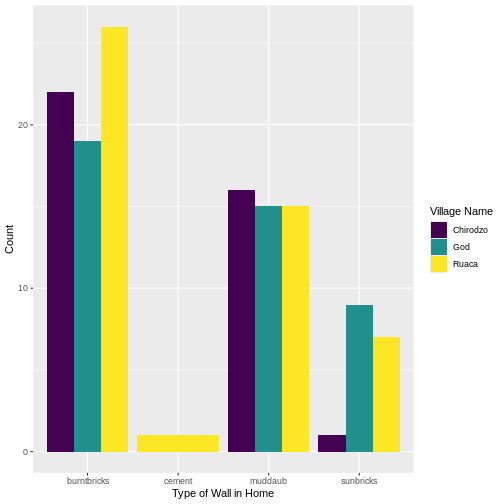
Other output options

---

You can convert R Markdown to a PDF or a Word document (among others). Click the little triangle next to the Knit button to get a drop-down menu. Or you could put pdf_document or word_document in the initial header of the file.

---
title: "My Awesome Report"
author: "Emmet Brickowski"
date: ""
output: word_document
---

Callout

Note: Creating PDF documents

Creating .pdf documents may require installation of some extra software. The R package tinytex provides some tools to help make this process easier for R users. With tinytex installed, run tinytex::install_tinytex() to install the required software (you’ll only need to do this once) and then when you Knit to pdf tinytex will automatically detect and install any additional LaTeX packages that are needed to produce the pdf document. Visit the tinytex website for more information.

Callout

Note: Inserting citations into an R Markdown file

It is possible to insert citations into an R Markdown file using the editor toolbar. The editor toolbar includes commonly seen formatting buttons generally seen in text editors (e.g., bold and italic buttons). The toolbar is accessible by using the settings dropdown menu (next to the ‘Knit’ dropdown menu) to select ‘Use Visual Editor’, also accessible through the shortcut ‘Crtl+Shift+F4’. From here, clicking ‘Insert’ allows ‘Citation’ to be selected (shortcut: ‘Crtl+Shift+F8’). For example, searching ‘10.1007/978-3-319-24277-4’ in ‘From DOI’ and inserting will provide the citation for ggplot2 [@wickham2016]. This will also save the citation(s) in ‘references.bib’ in the current working directory. Visit the R Studio website for more information. Tip: obtaining citation information from relevant packages can be done by using citation("package").

Resources

---

• Knitr in a knutshell tutorial
• Dynamic Documents with R and knitr (book)
• R Markdown documentation
• R Markdown cheat sheet
• Getting started with R Markdown
• Markdown tutorial
• R Markdown: The Definitive Guide (book by Rstudio team)
• Reproducible Reporting
• Introducing Bookdown

Key Points

• R Markdown is a useful language for creating reproducible documents combining text and executable R-code.
• Specify chunk options to control formatting of the output document

Content from Обробка даних JSON (необов'язково)

---

Last updated on 2026-01-19 | Edit this page

Estimated time: 45 minutes

Instructor Note

• Цей урок необов’язковий і призначений для ознайомлення з даними у форматі JSON, зокрема з тим, як зчитувати JSON у R та конвертувати ці дані у датафрейм або масив.
• Зауважте, що урок був створений спільнотою і досі знаходиться у процесі доопрацювання. Тому він може покращитися завдяки відгукам викладачів та/або учасників семінару.

Overview

Questions

• Що таке формат JSON?
• Як я можу перетворити JSON в датафрейм в R?
• Як я можу перетворити масив записів JSON у таблицю?

Objectives

• Опис формату даних JSON
• Розуміння, де JSON зазвичай використовується
• Оцініть деякі переваги використання JSON перед табличними даними
• Оцініть деякі недоліки обробки документів JSON
• Використовуйте пакет JSONLite для читання файлу JSON
• Відображення форматованого JSON як датафрейм
• Вибір та відображення вкладених полів датафрейму з документа JSON
• Запис табличних даних з вибраних елементів з документа JSON у файл csv

Формат даних JSON

---

The JSON data format was designed as a way of allowing different machines or processes within machines to communicate with each other by sending messages constructed in a well defined format. JSON is now the preferred data format used by APIs (Application Programming Interfaces).

The JSON format although somewhat verbose is not only Human readable but it can also be mapped very easily to an R dataframe.

We are going to read a file of data formatted as JSON, convert it into a dataframe in R then selectively create a csv file from the extracted data.

The JSON file we are going to use is the SAFI.json file. This is the output file from an electronic survey system called ODK. The JSON represents the answers to a series of survey questions. The questions themselves have been replaced with unique Keys, the values are the answers.

Because detailed surveys are by nature nested structures making it possible to record different levels of detail or selectively ask a set of specific questions based on the answer given to a previous question, the structure of the answers for the survey can not only be complex and convoluted, it could easily be different from one survey respondent’s set of answers to another.

Переваги JSON

• Very popular data format for APIs (e.g. results from an Internet search)
• Human readable
• Each record (or document as they are called) is self contained. The equivalent of the column name and column values are in every record.
• Documents do not all have to have the same structure within the same file
• Document structures can be complex and nested

Недоліки JSON

• It is more verbose than the equivalent data in csv format
• Can be more difficult to process and display than csv formatted data

Use the JSON package to read a JSON file

---

R

library(jsonlite)

As with reading in a CSV, you have a couple of options for how to access the JSON file.

You can read the JSON file directly into R with read_json() or the comparable fromJSON() function, though this does not download the file.

R

json_data <- read_json(
  "https://raw.githubusercontent.com/datacarpentry/r-socialsci/main/episodes/data/SAFI.json"
  )

To download the file you can copy and paste the contents of the file on GitHub, creating a SAFI.json file in your data directory, or you can download the file with R.

R

download.file(
  "https://raw.githubusercontent.com/datacarpentry/r-socialsci/main/episodes/data/SAFI.json",
   "data/SAFI.json", mode = "wb")

Once you have the data downloaded, you can read it into R with read_json():

R

json_data <- read_json("data/SAFI.json")

We can see that a new object called json_data has appeared in our Environment. It is described as a Large list (131 elements). In this current form, our data is messy. You can have a glimpse of it with the head() or view() functions. It will look not much more structured than if you were to open the JSON file with a text editor.

This is because, by default, the read_json() function’s parameter simplifyVector, which specifies whether or not to simplify vectors is set to FALSE. This means that the default setting does not simplify nested lists into vectors and data frames. However, we can set this to TRUE, and our data will be read directly as a dataframe:

R

json_data <- read_json("data/SAFI.json", simplifyVector = TRUE)

Now we can see we have this json data in a dataframe format. For consistency with the rest of the lesson, let’s coerce it to be a tibble and use glimpse to take a peek inside (these functions were loaded by library(tidyverse)):

R

json_data <- json_data %>% as_tibble()
glimpse(json_data)

OUTPUT

Rows: 131
Columns: 74
$ C06_rooms                      <int> 1, 1, 1, 1, 1, 1, 1, 3, 1, 5, 1, 3, 1, …
$ B19_grand_liv                  <chr> "no", "yes", "no", "no", "yes", "no", "…
$ A08_ward                       <chr> "ward2", "ward2", "ward2", "ward2", "wa…
$ E01_water_use                  <chr> "no", "yes", "no", "no", "no", "no", "y…
$ B18_sp_parents_liv             <chr> "yes", "yes", "no", "no", "no", "no", "…
$ B16_years_liv                  <int> 4, 9, 15, 6, 40, 3, 38, 70, 6, 23, 20, …
$ E_yes_group_count              <chr> NA, "3", NA, NA, NA, NA, "4", "2", "3",…
$ F_liv                          <list> [<data.frame[1 x 2]>], [<data.frame[3 …
$ `_note2`                       <lgl> NA, NA, NA, NA, NA, NA, NA, NA, NA, NA,…
$ instanceID                     <chr> "uuid:ec241f2c-0609-46ed-b5e8-fe575f6ce…
$ B20_sp_grand_liv               <chr> "yes", "yes", "no", "no", "no", "no", "…
$ F10_liv_owned_other            <lgl> NA, NA, NA, NA, NA, NA, NA, NA, NA, NA,…
$ `_note1`                       <lgl> NA, NA, NA, NA, NA, NA, NA, NA, NA, NA,…
$ F12_poultry                    <chr> "yes", "yes", "yes", "yes", "yes", "no"…
$ D_plots_count                  <chr> "2", "3", "1", "3", "2", "1", "4", "2",…
$ C02_respondent_wall_type_other <lgl> NA, NA, NA, NA, NA, NA, NA, NA, NA, NA,…
$ C02_respondent_wall_type       <chr> "muddaub", "muddaub", "burntbricks", "b…
$ C05_buildings_in_compound      <int> 1, 1, 1, 1, 1, 1, 1, 2, 2, 1, 2, 2, 1, …
$ `_remitters`                   <list> [<data.frame[0 x 0]>], [<data.frame[0 …
$ E18_months_no_water            <list> <NULL>, <"Aug", "Sept">, <NULL>, <NULL…
$ F07_use_income                 <chr> NA, "Alimentação e pagamento de educa…
$ G01_no_meals                   <int> 2, 2, 2, 2, 2, 2, 3, 2, 3, 3, 2, 3, 2, …
$ E17_no_enough_water            <chr> NA, "yes", NA, NA, NA, NA, "yes", "yes"…
$ F04_need_money                 <chr> NA, "no", NA, NA, NA, NA, "no", "no", "…
$ A05_end                        <chr> "2017-04-02T17:29:08.000Z", "2017-04-02…
$ C04_window_type                <chr> "no", "no", "yes", "no", "no", "no", "n…
$ E21_other_meth                 <chr> NA, "no", NA, NA, NA, NA, "no", "no", "…
$ D_no_plots                     <int> 2, 3, 1, 3, 2, 1, 4, 2, 3, 2, 2, 2, 4, …
$ F05_money_source               <list> <NULL>, <NULL>, <NULL>, <NULL>, <NULL>…
$ A07_district                   <chr> "district1", "district1", "district1", …
$ C03_respondent_floor_type      <chr> "earth", "earth", "cement", "earth", "e…
$ E_yes_group                    <list> [<data.frame[0 x 0]>], [<data.frame[3 …
$ A01_interview_date             <chr> "2016-11-17", "2016-11-17", "2016-11-17…
$ B11_remittance_money           <chr> "no", "no", "no", "no", "no", "no", "no…
$ A04_start                      <chr> "2017-03-23T09:49:57.000Z", "2017-04-02…
$ D_plots                        <list> [<data.frame[2 x 8]>], [<data.frame[3 …
$ F_items                        <list> [<data.frame[3 x 3]>], [<data.frame[2 …
$ F_liv_count                    <chr> "1", "3", "1", "2", "4", "1", "1", "2",…
$ F10_liv_owned                  <list> "poultry", <"oxen", "cows", "goats">, …
$ B_no_membrs                    <int> 3, 7, 10, 7, 7, 3, 6, 12, 8, 12, 6, 7, …
$ F13_du_look_aftr_cows          <chr> "no", "no", "no", "no", "no", "no", "no…
$ E26_affect_conflicts           <chr> NA, "once", NA, NA, NA, NA, "never", "n…
$ F14_items_owned                <list> <"bicycle", "television", "solar_panel…
$ F06_crops_contr                <chr> NA, "more_half", NA, NA, NA, NA, "more_…
$ B17_parents_liv                <chr> "no", "yes", "no", "no", "yes", "no", "…
$ G02_months_lack_food           <list> "Jan", <"Jan", "Sept", "Oct", "Nov", "…
$ A11_years_farm                 <dbl> 11, 2, 40, 6, 18, 3, 20, 16, 16, 22, 6,…
$ F09_du_labour                  <chr> "no", "no", "yes", "yes", "no", "yes", …
$ E_no_group_count               <chr> "2", NA, "1", "3", "2", "1", NA, NA, NA…
$ E22_res_change                 <list> <NULL>, <NULL>, <NULL>, <NULL>, <NULL>…
$ E24_resp_assoc                 <chr> NA, "no", NA, NA, NA, NA, NA, "yes", NA…
$ A03_quest_no                   <chr> "01", "01", "03", "04", "05", "6", "7",…
$ `_members`                     <list> [<data.frame[3 x 12]>], [<data.frame[7…
$ A06_province                   <chr> "province1", "province1", "province1", …
$ `gps:Accuracy`                 <dbl> 14, 19, 13, 5, 10, 12, 11, 9, 11, 14, 1…
$ E20_exper_other                <chr> NA, "yes", NA, NA, NA, NA, "yes", "yes"…
$ A09_village                    <chr> "village2", "village2", "village2", "vi…
$ C01_respondent_roof_type       <chr> "grass", "grass", "mabatisloping", "mab…
$ `gps:Altitude`                 <dbl> 698, 690, 674, 679, 689, 692, 709, 700,…
$ `gps:Longitude`                <dbl> 33.48346, 33.48342, 33.48345, 33.48342,…
$ E23_memb_assoc                 <chr> NA, "yes", NA, NA, NA, NA, "no", "yes",…
$ E19_period_use                 <dbl> NA, 2, NA, NA, NA, NA, 10, 10, 6, 22, N…
$ E25_fees_water                 <chr> NA, "no", NA, NA, NA, NA, "no", "no", "…
$ C07_other_buildings            <chr> "no", "no", "no", "no", "no", "no", "ye…
$ observation                    <chr> "None", "Estes primeiros inquéritos na…
$ `_note`                        <lgl> NA, NA, NA, NA, NA, NA, NA, NA, NA, NA,…
$ A12_agr_assoc                  <chr> "no", "yes", "no", "no", "no", "no", "n…
$ G03_no_food_mitigation         <list> <"na", "rely_less_food", "reduce_meals…
$ F05_money_source_other         <lgl> NA, NA, NA, NA, NA, NA, NA, NA, NA, NA,…
$ `gps:Latitude`                 <dbl> -19.11226, -19.11248, -19.11211, -19.11…
$ E_no_group                     <list> [<data.frame[2 x 6]>], [<data.frame[0 …
$ F14_items_owned_other          <lgl> NA, NA, NA, NA, NA, NA, NA, NA, NA, NA,…
$ F08_emply_lab                  <chr> "no", "yes", "no", "no", "no", "no", "n…
$ `_members_count`               <chr> "3", "7", "10", "7", "7", "3", "6", "12…

Looking good, but you might notice that actually we have a variable, F_liv that is a list of dataframes! It is very important to know what you are expecting from your data to be able to look for things like this. For example, if you are getting your JSON from an API, have a look at the API documentation, so you know what to look for.

Often when we have a very large number of columns, it can become difficult to determine all the variables which may require some special attention, like lists. Fortunately, we can use special verbs like where to quickly select all the list columns.

R

json_data %>%
    select(where(is.list)) %>%
    glimpse()

OUTPUT

Rows: 131
Columns: 14
$ F_liv                  <list> [<data.frame[1 x 2]>], [<data.frame[3 x 2]>], …
$ `_remitters`           <list> [<data.frame[0 x 0]>], [<data.frame[0 x 0]>], …
$ E18_months_no_water    <list> <NULL>, <"Aug", "Sept">, <NULL>, <NULL>, <NULL…
$ F05_money_source       <list> <NULL>, <NULL>, <NULL>, <NULL>, <NULL>, <NULL>…
$ E_yes_group            <list> [<data.frame[0 x 0]>], [<data.frame[3 x 14]>],…
$ D_plots                <list> [<data.frame[2 x 8]>], [<data.frame[3 x 8]>], …
$ F_items                <list> [<data.frame[3 x 3]>], [<data.frame[2 x 3]>], …
$ F10_liv_owned          <list> "poultry", <"oxen", "cows", "goats">, "none", …
$ F14_items_owned        <list> <"bicycle", "television", "solar_panel", "tabl…
$ G02_months_lack_food   <list> "Jan", <"Jan", "Sept", "Oct", "Nov", "Dec">, <…
$ E22_res_change         <list> <NULL>, <NULL>, <NULL>, <NULL>, <NULL>, <NULL>…
$ `_members`             <list> [<data.frame[3 x 12]>], [<data.frame[7 x 12]>]…
$ G03_no_food_mitigation <list> <"na", "rely_less_food", "reduce_meals", "day_…
$ E_no_group             <list> [<data.frame[2 x 6]>], [<data.frame[0 x 0]>], …

So what can we do about F_liv, the column of dataframes? Well first things first, we can access each one. For example to access the dataframe in the first row, we can use the bracket ([) subsetting. Here we use single bracket, but you could also use double bracket ([[). The [[ form allows only a single element to be selected using integer or character indices, whereas [ allows indexing by vectors.

R

json_data$F_liv[1]

OUTPUT

[[1]]
  F11_no_owned F_curr_liv
1            1    poultry

We can also choose to view the nested dataframes at all the rows of our main dataframe where a particular condition is met (for example where the value for the variable C06_rooms is equal to 4):

R

json_data$F_liv[which(json_data$C06_rooms == 4)]

OUTPUT

[[1]]
  F11_no_owned F_curr_liv
1            3       oxen
2            2       cows
3            5      goats

[[2]]
  F11_no_owned F_curr_liv
1            4       oxen
2            5       cows
3            3      goats

[[3]]
data frame with 0 columns and 0 rows

[[4]]
  F11_no_owned F_curr_liv
1            4       oxen
2            4       cows
3            4      goats
4            1      sheep

[[5]]
  F11_no_owned F_curr_liv
1            2       cows

Write the JSON file to csv

---

If we try to write our json_data dataframe to a csv as we would usually in a regular dataframe, we won’t get the desired result. Using the write_csv function from the readr package won’t give you an error for list columns, but you’ll only see missing (i.e. NA) values in these columns. Let’s try it out to confirm:

R

write_csv(json_data, "json_data_with_list_columns.csv")
read_csv("json_data_with_list_columns.csv")

To write out as a csv while maintaining the data within the list columns, we will need to “flatten” these columns. One way to do this is to convert these list columns into character types. (However, we don’t want to change the data types for any of the other columns). Here’s one way to do this using tidyverse. This command only applies the as.character command to those columns ‘where’ is.list is TRUE.

R

flattened_json_data <- json_data %>% 
  mutate(across(where(is.list), as.character))
flattened_json_data

OUTPUT

# A tibble: 131 × 74
   C06_rooms B19_grand_liv A08_ward E01_water_use B18_sp_parents_liv
       <int> <chr>         <chr>    <chr>         <chr>
 1         1 no            ward2    no            yes
 2         1 yes           ward2    yes           yes
 3         1 no            ward2    no            no
 4         1 no            ward2    no            no
 5         1 yes           ward2    no            no
 6         1 no            ward2    no            no
 7         1 yes           ward2    yes           no
 8         3 yes           ward1    yes           yes
 9         1 yes           ward2    yes           no
10         5 no            ward2    yes           no
# ℹ 121 more rows
# ℹ 69 more variables: B16_years_liv <int>, E_yes_group_count <chr>,
#   F_liv <chr>, `_note2` <lgl>, instanceID <chr>, B20_sp_grand_liv <chr>,
#   F10_liv_owned_other <lgl>, `_note1` <lgl>, F12_poultry <chr>,
#   D_plots_count <chr>, C02_respondent_wall_type_other <lgl>,
#   C02_respondent_wall_type <chr>, C05_buildings_in_compound <int>,
#   `_remitters` <chr>, E18_months_no_water <chr>, F07_use_income <chr>, …

Now you can write this to a csv file:

R

write_csv(flattened_json_data, "data_output/json_data_with_flattened_list_columns.csv")

Note: this means that when you read this csv back into R, the column of the nested dataframes will now be read in as a character vector. Converting it back to list to extract elements might be complicated, so it is probably better to keep storing these data in a JSON format if you will have to do this.

You can also write out the individual nested dataframes to a csv. Наприклад:

R

write_csv(json_data$F_liv[[1]], "data_output/F_liv_row1.csv")

Key Points

• JSON is a popular data format for transferring data used by a great many Web based APIs
• The complex structure of a JSON document means that it cannot easily be ‘flattened’ into tabular data
• We can use R code to extract values of interest and place them in a csv file